Predict Zero-inflated and Long/fat-tailed Outcomes

This notebook details how to predict a real-number outcome that is zero-inflated and long/fat-tailed such as sales prediction in retail. We provide baseline regression, regression trained using winsorized outcome, regression trained on log(y+1) outcome, and hurdle regression with and without Duan’s method.

Import

import pandas as pd
import numpy as np
import random
from ucimlrepo import fetch_ucirepo 
import boto3
import json
from tqdm.auto import tqdm
import time
from sklearn.model_selection import train_test_split
from autogluon.tabular import TabularDataset, TabularPredictor
from sklearn.metrics import (
    mean_squared_error, mean_absolute_error, r2_score, median_absolute_error,
    accuracy_score, precision_score, recall_score, f1_score, confusion_matrix
)

from scipy.stats import pearsonr, spearmanr, wasserstein_distance
from statsmodels.stats.diagnostic import het_white

def calculate_regression_metrics(y_true, y_pred):
    return {
        'root_mean_squared_error': np.sqrt(mean_squared_error(y_true, y_pred)),
        'mean_squared_error': mean_squared_error(y_true, y_pred),
        'mean_absolute_error': mean_absolute_error(y_true, y_pred),
        'r2': r2_score(y_true, y_pred),
        'pearsonr': pearsonr(y_true, y_pred)[0],  
        'spearmanr': spearmanr(y_true, y_pred)[0],
        'median_absolute_error': median_absolute_error(y_true, y_pred),
        'earths_mover_distance': wasserstein_distance(y_true, y_pred)
    }

def caluclate_classification_metrics(y_true, y_pred):
    return {
        'accuracy': accuracy_score(y_true, y_pred),
        'precision': precision_score(y_true, y_pred, average='weighted'),
        'recall': recall_score(y_true, y_pred, average='weighted'),
        'f1_score': f1_score(y_true, y_pred, average='weighted'),
        'confusion_matrix': confusion_matrix(y_true, y_pred)
    }

def string_to_yearmon(date):
    date = date.split()
    date = date[0].split('/') + date[1].split(':')
    date = date[2] + '-' + date[0].zfill(2) #+ '-' + date[1].zfill(2) + ' ' + date[3].zfill(2) + ':' + date[4].zfill(2)
    return date

def call_llama(system_prompt, input):
    template = f"""<s>[INST] <<SYS>>{system_prompt}<</SYS>>{input}[/INST]"""
    client = boto3.client(service_name='bedrock-runtime',region_name='us-west-2')
    body = json.dumps({
        "prompt": template,
        "temperature": 0.,
        "top_p": 0.9,
        "max_gen_len": 2048,
    })
    response = client.invoke_model(
        body=body,
        modelId='us.meta.llama3-2-90b-instruct-v1:0',
        accept='application/json',
        contentType='application/json'
    )
    response_body = json.loads(response['body'].read())
    return response_body

def call_claude(system_prompt, input):
    client = boto3.client(service_name='bedrock-runtime',region_name='us-west-2')
    body=json.dumps(
        {
            "anthropic_version": "bedrock-2023-05-31",
            "max_tokens": 2048,
            "messages": [
                {
                    "role": "user",
                    "content": [
                    {
                        "type": "text",
                        "text": system_prompt + '\n' + input,
                    }
                    ]
                }
                ]
        }  
    )  

    
    response = client.invoke_model(body=body, 
                                   modelId='anthropic.claude-3-5-sonnet-20241022-v2:0',
                                   contentType='application/json',
                                   accept='application/json')
    response_body = json.loads(response.get('body').read())
   
    return response_body

from sklearn.preprocessing import StandardScaler
from statsmodels.stats.outliers_influence import variance_inflation_factor
from statsmodels.tools.tools import add_constant

class Winsorizer:
    def __init__(self, cols, percentile=99):
        self.cols = cols  # List of columns to apply winsorization to
        self.percentile = percentile  # Percentile to define the outliers
        self.lower_bounds = {}  # To store the lower quantiles
        self.upper_bounds = {}  # To store the upper quantiles

    def fit(self, df):
        """Fit the winsorizer to the data, remembering the quantiles."""
        for col in self.cols:
            lower = df[col].quantile(1 - self.percentile / 100)
            upper = df[col].quantile(self.percentile / 100)
            self.lower_bounds[col] = lower
            self.upper_bounds[col] = upper
    
    def transform(self, df):
        """Apply winsorization to a new DataFrame using the learned quantiles."""
        for col in self.cols:
            lower = self.lower_bounds[col]
            upper = self.upper_bounds[col]
            df[col] = np.clip(df[col], lower, upper)
        return df

    def fit_transform(self, df):
        """Fit the model and apply winsorization to the same DataFrame."""
        self.fit(df)
        return self.transform(df)

def calculate_vif(df, cols):
    X = df[cols]
    X_with_const = add_constant(X)  # Add constant for VIF calculation
    vif_data = pd.DataFrame()
    vif_data['feature'] = X_with_const.columns
    vif_data['VIF'] = [variance_inflation_factor(X_with_const.values, i) for i in range(X_with_const.shape[1])]
    return vif_data

import seaborn as sns
import statsmodels.api as sm

Dataset

We use the UCI Online Retail dataset, which are transactions from a UK-based, non-store online retail from 2010-12-01 and 2011-12-09. We perform the following data processing:

1. Remove transactions without CustomerID; from 541,909 to 406,829 transactions
2. Filter out transactions where either UnitPrice or Quantity is less than zero; from 406,829 to 397,884 transactions
3. Fill in missing product Description with value UNKNOWN.

online_retail = fetch_ucirepo(id=352) 
transaction_df = online_retail['data']['original']
transaction_df.shape

(541909, 8)

#create yearmon for train-valid split
transaction_df['yearmon'] = transaction_df.InvoiceDate.map(string_to_yearmon)

#get rid of transactions without cid
transaction_df = transaction_df[~transaction_df.CustomerID.isna()].reset_index(drop=True)

#fill in unknown descriptions
transaction_df.Description = transaction_df.Description.fillna('UNKNOWN')

#convert customer id to string
transaction_df['CustomerID'] = transaction_df['CustomerID'].map(lambda x: str(int(x)))

transaction_df.shape

(406829, 9)

#check if still na
transaction_df.isna().mean()

InvoiceNo      0.0
StockCode      0.0
Description    0.0
Quantity       0.0
InvoiceDate    0.0
UnitPrice      0.0
CustomerID     0.0
Country        0.0
yearmon        0.0
dtype: float64

#simplify by filtering unit price and quantity to be non-zero (get rid of discounts, cancellations, etc)
transaction_df = transaction_df[(transaction_df.UnitPrice>0)&\
                                (transaction_df.Quantity>0)].reset_index(drop=True)
#add sales
transaction_df['Sales'] = transaction_df.UnitPrice * transaction_df.Quantity
transaction_df.shape

(397884, 10)

Problem Formulation and Outcome

We formulate the problem as predicting the sales (TargetSales) during Q4 2011 for each customers who bought at least one item during Q1-Q3 2011. Note that we are interested in predicting the actual sales number per customer as accurately as possible; this is common for marketing use cases such as determining what spend threshold to give each customer in a promotion, targeting customers for upselling, or detecting early signs of churns.

We transform the transaction dataset into a customer-level dataset where we calculate features using transactions between 2011-01 to 2011-09 and outcome using transactions between 2011-10 to 2011-12, summing Quantity times UnitPrice. We left-join the customers in feature set to outcome set. This will result in the zero-inflated nature of the outcome as not all customers will come back in Q4. The distribution of non-zero sales is naturally long/fat-tailed with a few customers having extraordinarily high amount of sales in Q4. This resulted in a customer-level dataset with 3,438 customers.

feature_period = {'start': '2011-01', 'end': '2011-09'}
outcome_period = {'start': '2011-10', 'end': '2011-12'}

feature_transaction = transaction_df[(transaction_df.yearmon>=feature_period['start'])&\
                                      (transaction_df.yearmon<=feature_period['end'])]
outcome_transaction = transaction_df[(transaction_df.yearmon>=outcome_period['start'])&\
                                      (transaction_df.yearmon<=outcome_period['end'])]
feature_transaction.shape, outcome_transaction.shape

((240338, 10), (131389, 10))

#aggregate sales during outcome period
outcome_sales = outcome_transaction.groupby('CustomerID').Sales.sum().reset_index()
outcome_sales

	CustomerID	Sales
0	12347	1519.14
1	12349	1757.55
2	12352	311.73
3	12356	58.35
4	12357	6207.67
...	...	...
2555	18276	335.86
2556	18277	110.38
2557	18282	77.84
2558	18283	974.21
2559	18287	1072.00

2560 rows × 2 columns

#aggregate sales during feature period
feature_sales = feature_transaction.groupby('CustomerID').Sales.sum().reset_index()
feature_sales

	CustomerID	Sales
0	12346	77183.60
1	12347	2079.07
2	12348	904.44
3	12350	334.40
4	12352	2194.31
...	...	...
3433	18280	180.60
3434	18281	80.82
3435	18282	100.21
3436	18283	1120.67
3437	18287	765.28

3438 rows × 2 columns

#merge to get TargetSales including those who spent during feature period but not during outcome (zeroes)
outcome_df = feature_sales[['CustomerID']].merge(outcome_sales, on='CustomerID', how='left')
outcome_df['Sales'] = outcome_df['Sales'].fillna(0)
outcome_df.columns = ['CustomerID', 'TargetSales']
outcome_df

	CustomerID	TargetSales
0	12346	0.00
1	12347	1519.14
2	12348	0.00
3	12350	0.00
4	12352	311.73
...	...	...
3433	18280	0.00
3434	18281	0.00
3435	18282	77.84
3436	18283	974.21
3437	18287	1072.00

3438 rows × 2 columns

#confirm zero-inflated, long/fat-tailed
outcome_df.TargetSales.describe(percentiles=[i/10 for i in range(10)])

count      3438.000000
mean        666.245829
std        4016.843037
min           0.000000
0%            0.000000
10%           0.000000
20%           0.000000
30%           0.000000
40%           0.000000
50%         102.005000
60%         263.006000
70%         425.790000
80%         705.878000
90%        1273.611000
max      168469.600000
Name: TargetSales, dtype: float64

#confirm zero-inflated, long/fat-tailed
outcome_df[outcome_df.TargetSales<=10_000].TargetSales.hist(bins=100)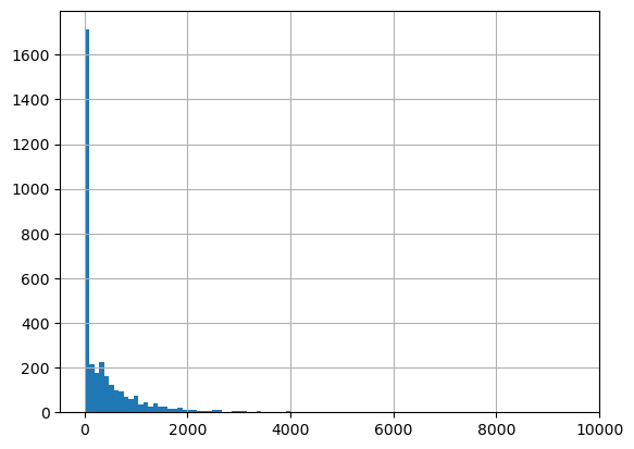

Feature

We represent a customer using traditional RFM features namely recency of purchase, purchase days, total sales, number of distinct products purchased, number of distinct category purchased, customer tenure within 2011, average purchase frequency, average purchase value, and percentage of purchase across all 9 categories. This is based on data from Q1-Q3 2011.

Since the UCI Online Retail dataset does not have a category but only contains descriptions over 3,000 items, we use LLaMA 3.2 90B to infer categories based on randomly selected 1,000 descriptions. This is to make the category preference representation for each customer, which is more tractable than including features about all 3,000+ items. After that, we use the same model to label a category for each description. The categories are:

1. Home Decor
2. Kitchen and Dining
3. Fashion Accessories
4. Stationary and Gifts
5. Toys and Games
6. Seasonal and Holiday
7. Personal Care and Wellness
8. Outdoor and Garden
9. Others

Classify Description into Category

feature_transaction.Description.nunique()

3548

Get Category

descriptions = feature_transaction.Description.unique().tolist()
print(descriptions[:5])

#randomize descriptions with seed 112 to get which categories we should use
np.random.seed(112)
random_descriptions = np.random.choice(descriptions, 1000, replace=False)
print(random_descriptions[:5])

['JUMBO BAG PINK POLKADOT', 'BLUE POLKADOT WRAP', 'RED RETROSPOT WRAP ', 'RECYCLING BAG RETROSPOT ', 'RED RETROSPOT SHOPPER BAG']
['MODERN FLORAL STATIONERY SET' 'PURPLE BERTIE GLASS BEAD BAG CHARM'
 'PARTY INVITES SPACEMAN' 'MONTANA DIAMOND CLUSTER EARRINGS'
 'SKULLS  DESIGN  COTTON TOTE BAG']

# res = call_llama(
#     'You are a product categorization assistant at a retail website.',
#     'Given the following product descriptions, come up with a few product categories they should be classified into.'+'\n'.join(random_descriptions)
#     )

# print(res['generation'])

# res

# res = call_claude(
#     'You are a product categorization assistant at a retail website.',
#     'Given the following product descriptions, come up with a few product categories they should be classified into.'+'\n'.join(random_descriptions)
#     )

# print(res['content'][0]['text'])

# res

LLaMA 3.2 90B Output:

<<SYS>>Based on the product descriptions, I would categorize them into the following categories:

1. Home Decor:
    * Wall art
    * Decorative items (e.g. vases, figurines, etc.)
    * Lighting (e.g. candles, lanterns, etc.)
    * Textiles (e.g. throw pillows, blankets, etc.)
2. Kitchen and Dining:
    * Cookware and utensils
    * Tableware (e.g. plates, cups, etc.)
    * Kitchen decor (e.g. signs, magnets, etc.)
    * Food and drink items (e.g. tea, coffee, etc.)
3. Fashion and Accessories:
    * Jewelry (e.g. necklaces, earrings, etc.)
    * Handbags and wallets
    * Clothing and accessories (e.g. scarves, hats, etc.)
4. Stationery and Gifts:
    * Cards and gift wrap
    * Stationery (e.g. notebooks, pens, etc.)
    * Gift items (e.g. mugs, keychains, etc.)
5. Toys and Games:
    * Toys (e.g. stuffed animals, puzzles, etc.)
    * Games and puzzles
6. Seasonal and Holiday:
    * Christmas decorations and gifts
    * Easter decorations and gifts
    * Other seasonal items (e.g. Halloween, etc.)
7. Personal Care and Wellness:
    * Beauty and personal care items (e.g. skincare, haircare, etc.)
    * Wellness and self-care items (e.g. essential oils, etc.)
8. Outdoor and Garden:
    * Garden decor and accessories
    * Outdoor furniture and decor
    * Gardening tools and supplies

Note that some products may fit into multiple categories, but I have assigned them to the one that seems most relevant.

Claude 3.5 v2 Output

Based on these product descriptions, I would suggest the following main product categories:

1. Home Decor
- Candle holders
- Picture frames
- Wall art & signs
- Clocks
- Cushions & covers
- Storage items
- Decorative objects

2. Jewelry & Accessories
- Necklaces
- Bracelets
- Earrings
- Hair accessories
- Bag charms
- Key rings

3. Garden & Outdoor
- Plant pots
- Garden tools
- Outdoor decorations
- Bird houses
- Garden markers

4. Kitchen & Dining
- Tea sets
- Mugs
- Kitchen storage
- Cutlery
- Baking accessories
- Tea towels

5. Stationery & Paper Goods
- Notebooks
- Gift wrap
- Cards
- Paper decorations
- Writing sets

6. Party & Celebrations
- Party supplies
- Gift bags
- Christmas decorations
- Easter items
- Birthday items

7. Children's Items
- Toys
- Children's tableware
- School supplies
- Kids' accessories

8. Fashion Accessories
- Bags
- Purses
- Scarves
- Travel accessories

9. Bath & Beauty
- Bathroom accessories
- Toiletry bags
- Beauty items

10. Lighting
- Lamps
- String lights
- Tea lights
- Lanterns

These categories cover the main types of products in the list while providing logical groupings for customers to browse.

categories = [
    'Home Decor',
    'Kitchen and Dining',
    'Fashion Accessories',
    'Stationary and Gifts',
    'Toys and Games',
    'Seasonal and Holiday',
    'Personal Care and Wellness',
    'Outdoor and Garden',   
]

len(categories)

8

Annotate Category to Description

# #loop through descriptions in batches of batch_size
# res_texts = []
# batch_size = 100
# for i in tqdm(range(0, len(descriptions), batch_size)):
#     batch = descriptions[i:i+batch_size]
#     d = "\n".join(batch)
#     inp = f'''Categorize the following product descriptions into {", ".join(categories)} or Others, if they do not fall into any. 
# Only answer in the following format:

# "product description of product #1"|"product category classified into"
# "product description of product #2"|"product category classified into"
# ...
# "product description of product #n"|"product category classified into"

# Here are the product descriptions:
# {d}
# '''
#     while True:
#         res = call_claude('You are a product categorizer at a retail website', inp)
#         # if res['generation_token_count'] > 1: #for llama
#         if res['usage']['output_tokens'] > 1:
#             break
#         else:
#             print('Retrying...')
#             time.sleep(2)
#     res_text = res['content'][0]['text'].strip().split('\n')
#         #for llama
#         # .replace('[SYS]','').replace('<<SYS>>','')\
#         # .replace('[/SYS]','').replace('<</SYS>>','')\
#     if res_text!='':
#         res_texts.extend(res_text)

# with open('../data/sales_prediction/product_description_category.csv','w') as f:
#     f.write('"product_description"|"category"\n')
#     for i in res_texts:
#         f.write(f'{i}\n')

product_description_category = pd.read_csv('../data/sales_prediction/product_description_category.csv',
                                           sep='|')

#clean product_description
product_description_category['Description'] = descriptions
product_description_category.category.value_counts(normalize=True)

category
Home Decor                    0.328636
Kitchen and Dining            0.195885
Fashion Accessories           0.138670
Stationary and Gifts          0.116122
Seasonal and Holiday          0.087373
Personal Care and Wellness    0.047351
Toys and Games                0.045096
Outdoor and Garden            0.032976
Others                        0.007892
Name: proportion, dtype: float64

feature_transaction_cat = feature_transaction.merge(product_description_category,
                                                    how='inner',
                                                    on = 'Description',)
feature_transaction.shape, feature_transaction_cat.shape

((240338, 10), (240338, 12))

RFM

#convert invoice date to datetime
feature_transaction_cat['InvoiceDate'] = pd.to_datetime(feature_transaction_cat['InvoiceDate'])

# last date in feature set
current_date = feature_transaction_cat['InvoiceDate'].max()

#rfm
customer_features = feature_transaction_cat.groupby('CustomerID').agg({
    'InvoiceDate': [
        ('recency', lambda x: (current_date - x.max()).days),
        ('first_purchase_date', 'min'),
        ('purchase_day', 'nunique'),
    ],
    'InvoiceNo': [('nb_invoice', 'nunique')],
    'Sales': [
        ('total_sales', 'sum')
    ],
    'StockCode': [('nb_product', 'nunique')],
    'category': [('nb_category', 'nunique')]
}).reset_index()

# Flatten column names
customer_features.columns = [
    'CustomerID',
    'recency',
    'first_purchase_date',
    'purchase_day',
    'nb_invoice',
    'total_sales',
    'nb_product',
    'nb_category'
]

#almost always one purchase a day
(customer_features.purchase_day==customer_features.nb_invoice).mean()

0.977021524141943

customer_features['customer_lifetime'] = (current_date - customer_features['first_purchase_date']).dt.days
customer_features['avg_purchase_frequency'] = customer_features['customer_lifetime'] / customer_features['purchase_day']
customer_features['avg_purchase_value'] = customer_features['total_sales'] / customer_features['purchase_day']

Category Preference

#category preference
category_sales = feature_transaction_cat.pivot_table(
    values='Sales', 
    index='CustomerID', 
    columns='category', 
    aggfunc='sum', 
    fill_value=0
)
category_sales.columns = [i.lower().replace(' ','_') for i in category_sales.columns]
customer_features = customer_features.merge(category_sales, on='CustomerID', how='left')

total_sales = customer_features['total_sales']
for col in category_sales.columns:
    percentage_col = f'per_{col}'
    customer_features[percentage_col] = customer_features[col] / total_sales

#make sure the categories are not too sparse
(customer_features.iloc[:,-9:]==0).mean()

per_fashion_accessories           0.409831
per_home_decor                    0.081734
per_kitchen_and_dining            0.122455
per_others                        0.765561
per_outdoor_and_garden            0.507853
per_personal_care_and_wellness    0.448226
per_seasonal_and_holiday          0.369401
per_stationary_and_gifts          0.305410
per_toys_and_games                0.487202
dtype: float64

Putting Them All Together

selected_features = [
 'recency',
 'purchase_day',
 'total_sales',
 'nb_product',
 'nb_category',
 'customer_lifetime',
 'avg_purchase_frequency',
 'avg_purchase_value',
 'per_fashion_accessories',
 'per_home_decor',
 'per_kitchen_and_dining',
 'per_others',
 'per_outdoor_and_garden',
 'per_personal_care_and_wellness',
 'per_seasonal_and_holiday',
 'per_stationary_and_gifts',
 'per_toys_and_games']

outcome_variable = 'TargetSales'

customer_features = customer_features[[ 'CustomerID']+selected_features]
customer_features.head()

	CustomerID	recency	purchase_day	total_sales	nb_product	nb_category	customer_lifetime	avg_purchase_frequency	avg_purchase_value	per_fashion_accessories	per_home_decor	per_kitchen_and_dining	per_others	per_outdoor_and_garden	per_personal_care_and_wellness	per_seasonal_and_holiday	per_stationary_and_gifts	per_toys_and_games
0	12346	255	1	77183.60	1	1	255	255.000000	77183.600000	0.000000	0.000000	1.000000	0.000000	0.000000	0.000000	0.000000	0.000000	0.000000
1	12347	59	4	2079.07	65	7	247	61.750000	519.767500	0.145834	0.204168	0.294021	0.000000	0.005628	0.147614	0.000000	0.073013	0.129721
2	12348	5	3	904.44	10	4	248	82.666667	301.480000	0.000000	0.000000	0.000000	0.132679	0.000000	0.825970	0.018796	0.022555	0.000000
3	12350	239	1	334.40	17	7	239	239.000000	334.400000	0.240431	0.202751	0.116926	0.172548	0.000000	0.118421	0.000000	0.059211	0.089713
4	12352	2	7	2194.31	47	8	226	32.285714	313.472857	0.000000	0.196531	0.246187	0.474090	0.013535	0.016680	0.008066	0.024404	0.020508

Merge Features and Outcome

customer_features.shape, outcome_df.shape

((3438, 18), (3438, 2))

df = outcome_df.merge(customer_features, on='CustomerID').drop('CustomerID', axis=1)
df.shape

(3438, 18)

#correlations
df.iloc[:,1:].corr()

	recency	purchase_day	total_sales	nb_product	nb_category	customer_lifetime	avg_purchase_frequency	avg_purchase_value	per_fashion_accessories	per_home_decor	per_kitchen_and_dining	per_others	per_outdoor_and_garden	per_personal_care_and_wellness	per_seasonal_and_holiday	per_stationary_and_gifts	per_toys_and_games
recency	1.000000	-0.299308	-0.132344	-0.287415	-0.326772	0.298853	0.893973	0.008823	-0.020861	0.022013	0.057244	-0.016069	0.071268	-0.082792	-0.085681	-0.017813	-0.009686
purchase_day	-0.299308	1.000000	0.540253	0.690345	0.304621	0.332109	-0.331543	0.027488	0.030683	0.018684	0.025269	0.004299	-0.019992	-0.035665	-0.020392	-0.045384	-0.028187
total_sales	-0.132344	0.540253	1.000000	0.400467	0.137064	0.156018	-0.148762	0.361138	0.016511	-0.013819	0.047834	0.006398	-0.029353	-0.011937	-0.016724	-0.029181	-0.013139
nb_product	-0.287415	0.690345	0.400467	1.000000	0.555551	0.265594	-0.294923	0.061039	-0.003137	-0.017516	0.035615	-0.006842	-0.026371	-0.005309	-0.016586	0.026716	-0.010069
nb_category	-0.326772	0.304621	0.137064	0.555551	1.000000	0.224232	-0.321596	0.019955	0.004863	-0.138372	-0.039363	0.055555	0.041405	0.075882	0.015498	0.152869	0.111150
customer_lifetime	0.298853	0.332109	0.156018	0.265594	0.224232	1.000000	0.358431	0.014933	0.011220	0.066111	0.069175	-0.019971	0.029726	-0.127865	-0.120399	-0.050320	-0.036484
avg_purchase_frequency	0.893973	-0.331543	-0.148762	-0.294923	-0.321596	0.358431	1.000000	0.009157	-0.016093	0.027208	0.037053	-0.027413	0.060369	-0.070352	-0.074799	-0.000546	-0.010612
avg_purchase_value	0.008823	0.027488	0.361138	0.061039	0.019955	0.014933	0.009157	1.000000	-0.003187	-0.056690	0.076862	0.015427	-0.028884	0.004225	-0.000200	-0.012729	-0.002396
per_fashion_accessories	-0.020861	0.030683	0.016511	-0.003137	0.004863	0.011220	-0.016093	-0.003187	1.000000	-0.254015	-0.177775	-0.010436	-0.082834	-0.038493	-0.124719	-0.068166	-0.051486
per_home_decor	0.022013	0.018684	-0.013819	-0.017516	-0.138372	0.066111	0.027208	-0.056690	-0.254015	1.000000	-0.481983	-0.155784	-0.080637	-0.158837	-0.165964	-0.262313	-0.245759
per_kitchen_and_dining	0.057244	0.025269	0.047834	0.035615	-0.039363	0.069175	0.037053	0.076862	-0.177775	-0.481983	1.000000	-0.013075	-0.144698	-0.117031	-0.204235	-0.173386	-0.143931
per_others	-0.016069	0.004299	0.006398	-0.006842	0.055555	-0.019971	-0.027413	0.015427	-0.010436	-0.155784	-0.013075	1.000000	-0.062652	0.014794	-0.047940	-0.033975	-0.040421
per_outdoor_and_garden	0.071268	-0.019992	-0.029353	-0.026371	0.041405	0.029726	0.060369	-0.028884	-0.082834	-0.080637	-0.144698	-0.062652	1.000000	-0.045639	-0.077947	-0.057297	-0.001034
per_personal_care_and_wellness	-0.082792	-0.035665	-0.011937	-0.005309	0.075882	-0.127865	-0.070352	0.004225	-0.038493	-0.158837	-0.117031	0.014794	-0.045639	1.000000	-0.057926	-0.025871	-0.017022
per_seasonal_and_holiday	-0.085681	-0.020392	-0.016724	-0.016586	0.015498	-0.120399	-0.074799	-0.000200	-0.124719	-0.165964	-0.204235	-0.047940	-0.077947	-0.057926	1.000000	-0.019418	-0.042970
per_stationary_and_gifts	-0.017813	-0.045384	-0.029181	0.026716	0.152869	-0.050320	-0.000546	-0.012729	-0.068166	-0.262313	-0.173386	-0.033975	-0.057297	-0.025871	-0.019418	1.000000	0.172039
per_toys_and_games	-0.009686	-0.028187	-0.013139	-0.010069	0.111150	-0.036484	-0.010612	-0.002396	-0.051486	-0.245759	-0.143931	-0.040421	-0.001034	-0.017022	-0.042970	0.172039	1.000000

#target and most predictive variable
df[df.TargetSales<=25_000].plot.scatter(x='TargetSales',y='total_sales')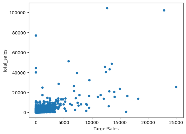

Train-Test Splits

We randomly split the dataset into train and test sets at 80/20 ratio. We also confirm the distribution of TargetSales is similar across percentiles and only different at the upper end.

#split into train-valid sets
train_df, test_df = train_test_split(df,
                                      test_size=0.2, 
                                      random_state=112)

pd.concat([train_df.TargetSales.describe(percentiles=[i/10 for i in range(10)]).reset_index(),
test_df.TargetSales.describe(percentiles=[i/10 for i in range(10)]).reset_index(),], axis=1)

	index	TargetSales	index	TargetSales
0	count	2750.000000	count	688.000000
1	mean	642.650436	mean	760.558808
2	std	4015.305436	std	4024.524400
3	min	0.000000	min	0.000000
4	0%	0.000000	0%	0.000000
5	10%	0.000000	10%	0.000000
6	20%	0.000000	20%	0.000000
7	30%	0.000000	30%	0.000000
8	40%	0.000000	40%	0.000000
9	50%	91.350000	50%	113.575000
10	60%	260.308000	60%	277.836000
11	70%	426.878000	70%	418.187000
12	80%	694.164000	80%	759.582000
13	90%	1272.997000	90%	1255.670000
14	max	168469.600000	max	77099.380000

Baseline Regression

The most naive solution is to predict TargetSales based on the features. We use a stacked ensemble of LightGBM, CatBoost, XGBoost, Random Forest and Extra Trees via AutoGluon. We train with good_quality preset, stated to be “Stronger than any other AutoML Framework”, for speedy training and inference but feel free to try more performant option. We exclude the neural-network models as they require further preprocessing of the features.

We use an industry-grade, non-parametric model to be as close to a real use case as possible and make a point that our methodology works not only in a toy-dataset setup.

preset = 'good_quality'

predictor = TabularPredictor(label='TargetSales').fit(train_df[selected_features + ['TargetSales']], 
                                                      presets=preset,
                                                      excluded_model_types=['NN_TORCH','FASTAI','KNN'],
                                                      )

No path specified. Models will be saved in: "AutogluonModels/ag-20241214_134505"
Verbosity: 2 (Standard Logging)
=================== System Info ===================
AutoGluon Version:  1.1.1
Python Version:     3.9.12
Operating System:   Linux
Platform Machine:   x86_64
Platform Version:   #1 SMP Wed Oct 23 01:22:11 UTC 2024
CPU Count:          64
Memory Avail:       470.24 GB / 480.23 GB (97.9%)
Disk Space Avail:   1451.64 GB / 1968.52 GB (73.7%)
===================================================
Presets specified: ['good_quality']
Setting dynamic_stacking from 'auto' to True. Reason: Enable dynamic_stacking when use_bag_holdout is disabled. (use_bag_holdout=False)
Stack configuration (auto_stack=True): num_stack_levels=1, num_bag_folds=8, num_bag_sets=1
Note: `save_bag_folds=False`! This will greatly reduce peak disk usage during fit (by ~8x), but runs the risk of an out-of-memory error during model refit if memory is small relative to the data size.
    You can avoid this risk by setting `save_bag_folds=True`.
DyStack is enabled (dynamic_stacking=True). AutoGluon will try to determine whether the input data is affected by stacked overfitting and enable or disable stacking as a consequence.
    This is used to identify the optimal `num_stack_levels` value. Copies of AutoGluon will be fit on subsets of the data. Then holdout validation data is used to detect stacked overfitting.
    Running DyStack for up to 900s of the 3600s of remaining time (25%).
2024-12-14 13:45:05,288 INFO util.py:154 -- Outdated packages:
  ipywidgets==7.6.5 found, needs ipywidgets>=8
Run `pip install -U ipywidgets`, then restart the notebook server for rich notebook output.
/home/charipol/miniconda3/lib/python3.9/site-packages/autogluon/tabular/predictor/predictor.py:1242: UserWarning: Failed to use ray for memory safe fits. Falling back to normal fit. Error: ValueError('ray==2.40.0 detected. 2.10.0 <= ray < 2.11.0 is required. You can use pip to install certain version of ray `pip install ray==2.10.0` ')
  stacked_overfitting = self._sub_fit_memory_save_wrapper(
        Context path: "AutogluonModels/ag-20241214_134505/ds_sub_fit/sub_fit_ho"
Running DyStack sub-fit ...
Beginning AutoGluon training ... Time limit = 900s
AutoGluon will save models to "AutogluonModels/ag-20241214_134505/ds_sub_fit/sub_fit_ho"
Train Data Rows:    2444
Train Data Columns: 17
Label Column:       TargetSales
Problem Type:       regression
Preprocessing data ...
Using Feature Generators to preprocess the data ...
Fitting AutoMLPipelineFeatureGenerator...
    Available Memory:                    481515.82 MB
    Train Data (Original)  Memory Usage: 0.32 MB (0.0% of available memory)
    Inferring data type of each feature based on column values. Set feature_metadata_in to manually specify special dtypes of the features.
    Stage 1 Generators:
        Fitting AsTypeFeatureGenerator...
    Stage 2 Generators:
        Fitting FillNaFeatureGenerator...
    Stage 3 Generators:
        Fitting IdentityFeatureGenerator...
    Stage 4 Generators:
        Fitting DropUniqueFeatureGenerator...
    Stage 5 Generators:
        Fitting DropDuplicatesFeatureGenerator...
    Types of features in original data (raw dtype, special dtypes):
        ('float', []) : 12 | ['total_sales', 'avg_purchase_frequency', 'avg_purchase_value', 'per_fashion_accessories', 'per_home_decor', ...]
        ('int', [])   :  5 | ['recency', 'purchase_day', 'nb_product', 'nb_category', 'customer_lifetime']
    Types of features in processed data (raw dtype, special dtypes):
        ('float', []) : 12 | ['total_sales', 'avg_purchase_frequency', 'avg_purchase_value', 'per_fashion_accessories', 'per_home_decor', ...]
        ('int', [])   :  5 | ['recency', 'purchase_day', 'nb_product', 'nb_category', 'customer_lifetime']
    0.0s = Fit runtime
    17 features in original data used to generate 17 features in processed data.
    Train Data (Processed) Memory Usage: 0.32 MB (0.0% of available memory)
Data preprocessing and feature engineering runtime = 0.06s ...
AutoGluon will gauge predictive performance using evaluation metric: 'root_mean_squared_error'
    This metric's sign has been flipped to adhere to being higher_is_better. The metric score can be multiplied by -1 to get the metric value.
    To change this, specify the eval_metric parameter of Predictor()
User-specified model hyperparameters to be fit:
{
    'NN_TORCH': {},
    'GBM': [{'extra_trees': True, 'ag_args': {'name_suffix': 'XT'}}, {}, 'GBMLarge'],
    'CAT': {},
    'XGB': {},
    'FASTAI': {},
    'RF': [{'criterion': 'gini', 'max_depth': 15, 'ag_args': {'name_suffix': 'Gini', 'problem_types': ['binary', 'multiclass']}}, {'criterion': 'entropy', 'max_depth': 15, 'ag_args': {'name_suffix': 'Entr', 'problem_types': ['binary', 'multiclass']}}, {'criterion': 'squared_error', 'max_depth': 15, 'ag_args': {'name_suffix': 'MSE', 'problem_types': ['regression', 'quantile']}}],
    'XT': [{'criterion': 'gini', 'max_depth': 15, 'ag_args': {'name_suffix': 'Gini', 'problem_types': ['binary', 'multiclass']}}, {'criterion': 'entropy', 'max_depth': 15, 'ag_args': {'name_suffix': 'Entr', 'problem_types': ['binary', 'multiclass']}}, {'criterion': 'squared_error', 'max_depth': 15, 'ag_args': {'name_suffix': 'MSE', 'problem_types': ['regression', 'quantile']}}],
}
AutoGluon will fit 2 stack levels (L1 to L2) ...
Excluded models: ['NN_TORCH', 'FASTAI'] (Specified by `excluded_model_types`)
Fitting 7 L1 models ...
Fitting model: LightGBMXT_BAG_L1 ... Training model for up to 599.62s of the 899.66s of remaining time.
Will use sequential fold fitting strategy because import of ray failed. Reason: ray==2.40.0 detected. 2.10.0 <= ray < 2.11.0 is required. You can use pip to install certain version of ray `pip install ray==2.10.0` 
    Fitting 8 child models (S1F1 - S1F8) | Fitting with SequentialLocalFoldFittingStrategy
    -3990.4801   = Validation score   (-root_mean_squared_error)
    6.36s    = Training   runtime
    0.01s    = Validation runtime
Fitting model: LightGBM_BAG_L1 ... Training model for up to 593.17s of the 893.2s of remaining time.
    Fitting 8 child models (S1F1 - S1F8) | Fitting with SequentialLocalFoldFittingStrategy
    -3921.7042   = Validation score   (-root_mean_squared_error)
    5.31s    = Training   runtime
    0.01s    = Validation runtime
Fitting model: RandomForestMSE_BAG_L1 ... Training model for up to 587.75s of the 887.78s of remaining time.
    -4516.1791   = Validation score   (-root_mean_squared_error)
    0.89s    = Training   runtime
    0.17s    = Validation runtime
Fitting model: CatBoost_BAG_L1 ... Training model for up to 586.59s of the 886.62s of remaining time.
    Fitting 8 child models (S1F1 - S1F8) | Fitting with SequentialLocalFoldFittingStrategy
    -3857.3111   = Validation score   (-root_mean_squared_error)
    10.49s   = Training   runtime
    0.02s    = Validation runtime
Fitting model: ExtraTreesMSE_BAG_L1 ... Training model for up to 575.99s of the 876.03s of remaining time.
    -3900.3038   = Validation score   (-root_mean_squared_error)
    0.66s    = Training   runtime
    0.17s    = Validation runtime
Fitting model: XGBoost_BAG_L1 ... Training model for up to 575.08s of the 875.11s of remaining time.
    Fitting 8 child models (S1F1 - S1F8) | Fitting with SequentialLocalFoldFittingStrategy
    -3941.3599   = Validation score   (-root_mean_squared_error)
    6.1s     = Training   runtime
    0.03s    = Validation runtime
Fitting model: LightGBMLarge_BAG_L1 ... Training model for up to 568.89s of the 868.93s of remaining time.
    Fitting 8 child models (S1F1 - S1F8) | Fitting with SequentialLocalFoldFittingStrategy
    -3912.54     = Validation score   (-root_mean_squared_error)
    12.28s   = Training   runtime
    0.01s    = Validation runtime
Fitting model: WeightedEnsemble_L2 ... Training model for up to 360.0s of the 856.55s of remaining time.
    Ensemble Weights: {'CatBoost_BAG_L1': 0.6, 'ExtraTreesMSE_BAG_L1': 0.36, 'LightGBM_BAG_L1': 0.04}
    -3835.4224   = Validation score   (-root_mean_squared_error)
    0.02s    = Training   runtime
    0.0s     = Validation runtime
Excluded models: ['NN_TORCH', 'FASTAI'] (Specified by `excluded_model_types`)
Fitting 7 L2 models ...
Fitting model: LightGBMXT_BAG_L2 ... Training model for up to 856.47s of the 856.47s of remaining time.
    Fitting 8 child models (S1F1 - S1F8) | Fitting with SequentialLocalFoldFittingStrategy
    -3941.7891   = Validation score   (-root_mean_squared_error)
    4.54s    = Training   runtime
    0.01s    = Validation runtime
Fitting model: LightGBM_BAG_L2 ... Training model for up to 851.87s of the 851.86s of remaining time.
    Fitting 8 child models (S1F1 - S1F8) | Fitting with SequentialLocalFoldFittingStrategy

[1000]  valid_set's rmse: 4314.99

    -3894.7078   = Validation score   (-root_mean_squared_error)
    5.58s    = Training   runtime
    0.01s    = Validation runtime
Fitting model: RandomForestMSE_BAG_L2 ... Training model for up to 846.2s of the 846.19s of remaining time.
    -4525.2057   = Validation score   (-root_mean_squared_error)
    0.87s    = Training   runtime
    0.17s    = Validation runtime
Fitting model: CatBoost_BAG_L2 ... Training model for up to 845.08s of the 845.07s of remaining time.
    Fitting 8 child models (S1F1 - S1F8) | Fitting with SequentialLocalFoldFittingStrategy
    -3904.7749   = Validation score   (-root_mean_squared_error)
    5.45s    = Training   runtime
    0.02s    = Validation runtime
Fitting model: ExtraTreesMSE_BAG_L2 ... Training model for up to 839.51s of the 839.5s of remaining time.
    -3952.2022   = Validation score   (-root_mean_squared_error)
    0.68s    = Training   runtime
    0.17s    = Validation runtime
Fitting model: XGBoost_BAG_L2 ... Training model for up to 838.57s of the 838.56s of remaining time.
    Fitting 8 child models (S1F1 - S1F8) | Fitting with SequentialLocalFoldFittingStrategy
    -3929.2019   = Validation score   (-root_mean_squared_error)
    6.6s     = Training   runtime
    0.04s    = Validation runtime
Fitting model: LightGBMLarge_BAG_L2 ... Training model for up to 831.87s of the 831.86s of remaining time.
    Fitting 8 child models (S1F1 - S1F8) | Fitting with SequentialLocalFoldFittingStrategy
    -3912.6409   = Validation score   (-root_mean_squared_error)
    13.59s   = Training   runtime
    0.01s    = Validation runtime
Fitting model: WeightedEnsemble_L3 ... Training model for up to 360.0s of the 818.17s of remaining time.
    Ensemble Weights: {'CatBoost_BAG_L1': 0.36, 'ExtraTreesMSE_BAG_L1': 0.32, 'LightGBM_BAG_L2': 0.32}
    -3823.1639   = Validation score   (-root_mean_squared_error)
    0.03s    = Training   runtime
    0.0s     = Validation runtime
AutoGluon training complete, total runtime = 81.64s ... Best model: WeightedEnsemble_L3 | Estimated inference throughput: 2283.2 rows/s (306 batch size)
Automatically performing refit_full as a post-fit operation (due to `.fit(..., refit_full=True)`
Refitting models via `predictor.refit_full` using all of the data (combined train and validation)...
    Models trained in this way will have the suffix "_FULL" and have NaN validation score.
    This process is not bound by time_limit, but should take less time than the original `predictor.fit` call.
    To learn more, refer to the `.refit_full` method docstring which explains how "_FULL" models differ from normal models.
Fitting 1 L1 models ...
Fitting model: LightGBMXT_BAG_L1_FULL ...
    0.25s    = Training   runtime
Fitting 1 L1 models ...
Fitting model: LightGBM_BAG_L1_FULL ...
    0.21s    = Training   runtime
Fitting model: RandomForestMSE_BAG_L1_FULL | Skipping fit via cloning parent ...
    0.89s    = Training   runtime
    0.17s    = Validation runtime
Fitting 1 L1 models ...
Fitting model: CatBoost_BAG_L1_FULL ...
    0.6s     = Training   runtime
Fitting model: ExtraTreesMSE_BAG_L1_FULL | Skipping fit via cloning parent ...
    0.66s    = Training   runtime
    0.17s    = Validation runtime
Fitting 1 L1 models ...
Fitting model: XGBoost_BAG_L1_FULL ...
    0.12s    = Training   runtime
Fitting 1 L1 models ...
Fitting model: LightGBMLarge_BAG_L1_FULL ...
    0.34s    = Training   runtime
Fitting model: WeightedEnsemble_L2_FULL | Skipping fit via cloning parent ...
    Ensemble Weights: {'CatBoost_BAG_L1': 0.6, 'ExtraTreesMSE_BAG_L1': 0.36, 'LightGBM_BAG_L1': 0.04}
    0.02s    = Training   runtime
Fitting 1 L2 models ...
Fitting model: LightGBMXT_BAG_L2_FULL ...
    0.21s    = Training   runtime
Fitting 1 L2 models ...
Fitting model: LightGBM_BAG_L2_FULL ...
    0.31s    = Training   runtime
Fitting model: RandomForestMSE_BAG_L2_FULL | Skipping fit via cloning parent ...
    0.87s    = Training   runtime
    0.17s    = Validation runtime
Fitting 1 L2 models ...
Fitting model: CatBoost_BAG_L2_FULL ...
    0.17s    = Training   runtime
Fitting model: ExtraTreesMSE_BAG_L2_FULL | Skipping fit via cloning parent ...
    0.68s    = Training   runtime
    0.17s    = Validation runtime
Fitting 1 L2 models ...
Fitting model: XGBoost_BAG_L2_FULL ...
    0.19s    = Training   runtime
Fitting 1 L2 models ...
Fitting model: LightGBMLarge_BAG_L2_FULL ...
    0.43s    = Training   runtime
Fitting model: WeightedEnsemble_L3_FULL | Skipping fit via cloning parent ...
    Ensemble Weights: {'CatBoost_BAG_L1': 0.36, 'ExtraTreesMSE_BAG_L1': 0.32, 'LightGBM_BAG_L2': 0.32}
    0.03s    = Training   runtime
Updated best model to "WeightedEnsemble_L3_FULL" (Previously "WeightedEnsemble_L3"). AutoGluon will default to using "WeightedEnsemble_L3_FULL" for predict() and predict_proba().
Refit complete, total runtime = 3.45s ... Best model: "WeightedEnsemble_L3_FULL"
TabularPredictor saved. To load, use: predictor = TabularPredictor.load("AutogluonModels/ag-20241214_134505/ds_sub_fit/sub_fit_ho")
Deleting DyStack predictor artifacts (clean_up_fits=True) ...
Leaderboard on holdout data (DyStack):
                          model  score_holdout    score_val              eval_metric  pred_time_test  pred_time_val  fit_time  pred_time_test_marginal  pred_time_val_marginal  fit_time_marginal  stack_level  can_infer  fit_order
0          CatBoost_BAG_L1_FULL    -803.899801 -3857.311112  root_mean_squared_error        0.006679            NaN  0.597072                 0.006679                     NaN           0.597072            1       True          4
1      WeightedEnsemble_L2_FULL    -813.259482 -3835.422447  root_mean_squared_error        0.120649            NaN  1.485833                 0.002517                     NaN           0.018860            2       True          8
2          CatBoost_BAG_L2_FULL    -838.233626 -3904.774934  root_mean_squared_error        0.258556            NaN  3.238374                 0.006184                     NaN           0.173173            2       True         12
3   RandomForestMSE_BAG_L1_FULL    -847.825565 -4516.179095  root_mean_squared_error        0.113628       0.174859  0.894842                 0.113628                0.174859           0.894842            1       True          3
4     ExtraTreesMSE_BAG_L2_FULL    -890.912998 -3952.202176  root_mean_squared_error        0.360469            NaN  3.743573                 0.108097                0.171160           0.678372            2       True         13
5     ExtraTreesMSE_BAG_L1_FULL    -922.896541 -3900.303809  root_mean_squared_error        0.109015       0.173588  0.658955                 0.109015                0.173588           0.658955            1       True          5
6      WeightedEnsemble_L3_FULL    -977.887954 -3823.163850  root_mean_squared_error        0.260014            NaN  3.409128                 0.003530                     NaN           0.031533            3       True         16
7          LightGBM_BAG_L1_FULL   -1086.123687 -3921.704247  root_mean_squared_error        0.002438            NaN  0.210945                 0.002438                     NaN           0.210945            1       True          2
8   RandomForestMSE_BAG_L2_FULL   -1090.066132 -4525.205744  root_mean_squared_error        0.349192            NaN  3.933684                 0.096820                0.174712           0.868483            2       True         11
9        LightGBMXT_BAG_L1_FULL   -1230.340360 -3990.480139  root_mean_squared_error        0.002607            NaN  0.245293                 0.002607                     NaN           0.245293            1       True          1
10       LightGBMXT_BAG_L2_FULL   -1234.815155 -3941.789134  root_mean_squared_error        0.255407            NaN  3.276018                 0.003035                     NaN           0.210817            2       True          9
11    LightGBMLarge_BAG_L1_FULL   -1345.024278 -3912.540001  root_mean_squared_error        0.004740            NaN  0.335057                 0.004740                     NaN           0.335057            1       True          7
12    LightGBMLarge_BAG_L2_FULL   -1640.347524 -3912.640942  root_mean_squared_error        0.262513            NaN  3.497248                 0.010141                     NaN           0.432046            2       True         15
13         LightGBM_BAG_L2_FULL   -1743.255667 -3894.707823  root_mean_squared_error        0.256483            NaN  3.377595                 0.004111                     NaN           0.312394            2       True         10
14          XGBoost_BAG_L1_FULL   -2245.433966 -3941.359884  root_mean_squared_error        0.013265            NaN  0.123036                 0.013265                     NaN           0.123036            1       True          6
15          XGBoost_BAG_L2_FULL   -2454.083373 -3929.201875  root_mean_squared_error        0.267445            NaN  3.256454                 0.015073                     NaN           0.191253            2       True         14
    0    = Optimal   num_stack_levels (Stacked Overfitting Occurred: True)
    86s  = DyStack   runtime |  3514s    = Remaining runtime
Starting main fit with num_stack_levels=0.
    For future fit calls on this dataset, you can skip DyStack to save time: `predictor.fit(..., dynamic_stacking=False, num_stack_levels=0)`
Beginning AutoGluon training ... Time limit = 3514s
AutoGluon will save models to "AutogluonModels/ag-20241214_134505"
Train Data Rows:    2750
Train Data Columns: 17
Label Column:       TargetSales
Problem Type:       regression
Preprocessing data ...
Using Feature Generators to preprocess the data ...
Fitting AutoMLPipelineFeatureGenerator...
    Available Memory:                    480433.27 MB
    Train Data (Original)  Memory Usage: 0.36 MB (0.0% of available memory)
    Inferring data type of each feature based on column values. Set feature_metadata_in to manually specify special dtypes of the features.
    Stage 1 Generators:
        Fitting AsTypeFeatureGenerator...
    Stage 2 Generators:
        Fitting FillNaFeatureGenerator...
    Stage 3 Generators:
        Fitting IdentityFeatureGenerator...
    Stage 4 Generators:
        Fitting DropUniqueFeatureGenerator...
    Stage 5 Generators:
        Fitting DropDuplicatesFeatureGenerator...
    Types of features in original data (raw dtype, special dtypes):
        ('float', []) : 12 | ['total_sales', 'avg_purchase_frequency', 'avg_purchase_value', 'per_fashion_accessories', 'per_home_decor', ...]
        ('int', [])   :  5 | ['recency', 'purchase_day', 'nb_product', 'nb_category', 'customer_lifetime']
    Types of features in processed data (raw dtype, special dtypes):
        ('float', []) : 12 | ['total_sales', 'avg_purchase_frequency', 'avg_purchase_value', 'per_fashion_accessories', 'per_home_decor', ...]
        ('int', [])   :  5 | ['recency', 'purchase_day', 'nb_product', 'nb_category', 'customer_lifetime']
    0.1s = Fit runtime
    17 features in original data used to generate 17 features in processed data.
    Train Data (Processed) Memory Usage: 0.36 MB (0.0% of available memory)
Data preprocessing and feature engineering runtime = 0.08s ...
AutoGluon will gauge predictive performance using evaluation metric: 'root_mean_squared_error'
    This metric's sign has been flipped to adhere to being higher_is_better. The metric score can be multiplied by -1 to get the metric value.
    To change this, specify the eval_metric parameter of Predictor()
User-specified model hyperparameters to be fit:
{
    'NN_TORCH': {},
    'GBM': [{'extra_trees': True, 'ag_args': {'name_suffix': 'XT'}}, {}, 'GBMLarge'],
    'CAT': {},
    'XGB': {},
    'FASTAI': {},
    'RF': [{'criterion': 'gini', 'max_depth': 15, 'ag_args': {'name_suffix': 'Gini', 'problem_types': ['binary', 'multiclass']}}, {'criterion': 'entropy', 'max_depth': 15, 'ag_args': {'name_suffix': 'Entr', 'problem_types': ['binary', 'multiclass']}}, {'criterion': 'squared_error', 'max_depth': 15, 'ag_args': {'name_suffix': 'MSE', 'problem_types': ['regression', 'quantile']}}],
    'XT': [{'criterion': 'gini', 'max_depth': 15, 'ag_args': {'name_suffix': 'Gini', 'problem_types': ['binary', 'multiclass']}}, {'criterion': 'entropy', 'max_depth': 15, 'ag_args': {'name_suffix': 'Entr', 'problem_types': ['binary', 'multiclass']}}, {'criterion': 'squared_error', 'max_depth': 15, 'ag_args': {'name_suffix': 'MSE', 'problem_types': ['regression', 'quantile']}}],
}
Excluded models: ['NN_TORCH', 'FASTAI'] (Specified by `excluded_model_types`)
Fitting 7 L1 models ...
Fitting model: LightGBMXT_BAG_L1 ... Training model for up to 3513.91s of the 3513.9s of remaining time.
    Fitting 8 child models (S1F1 - S1F8) | Fitting with SequentialLocalFoldFittingStrategy

[1000]  valid_set's rmse: 9800.07
[2000]  valid_set's rmse: 9792.42
[3000]  valid_set's rmse: 9791.47

    -3713.1197   = Validation score   (-root_mean_squared_error)
    8.47s    = Training   runtime
    0.01s    = Validation runtime
Fitting model: LightGBM_BAG_L1 ... Training model for up to 3505.33s of the 3505.33s of remaining time.
    Fitting 8 child models (S1F1 - S1F8) | Fitting with SequentialLocalFoldFittingStrategy

[1000]  valid_set's rmse: 9561.64
[2000]  valid_set's rmse: 9538.68

    -3635.1505   = Validation score   (-root_mean_squared_error)
    6.15s    = Training   runtime
    0.01s    = Validation runtime
Fitting model: RandomForestMSE_BAG_L1 ... Training model for up to 3499.08s of the 3499.08s of remaining time.
    -4135.0334   = Validation score   (-root_mean_squared_error)
    0.82s    = Training   runtime
    0.18s    = Validation runtime
Fitting model: CatBoost_BAG_L1 ... Training model for up to 3497.99s of the 3497.99s of remaining time.
    Fitting 8 child models (S1F1 - S1F8) | Fitting with SequentialLocalFoldFittingStrategy
    -3669.0125   = Validation score   (-root_mean_squared_error)
    18.54s   = Training   runtime
    0.02s    = Validation runtime
Fitting model: ExtraTreesMSE_BAG_L1 ... Training model for up to 3479.34s of the 3479.34s of remaining time.
    -3678.3921   = Validation score   (-root_mean_squared_error)
    0.66s    = Training   runtime
    0.18s    = Validation runtime
Fitting model: XGBoost_BAG_L1 ... Training model for up to 3478.41s of the 3478.41s of remaining time.
    Fitting 8 child models (S1F1 - S1F8) | Fitting with SequentialLocalFoldFittingStrategy
    -3785.5048   = Validation score   (-root_mean_squared_error)
    5.79s    = Training   runtime
    0.04s    = Validation runtime
Fitting model: LightGBMLarge_BAG_L1 ... Training model for up to 3472.52s of the 3472.51s of remaining time.
    Fitting 8 child models (S1F1 - S1F8) | Fitting with SequentialLocalFoldFittingStrategy
    -3704.5742   = Validation score   (-root_mean_squared_error)
    11.91s   = Training   runtime
    0.01s    = Validation runtime
Fitting model: WeightedEnsemble_L2 ... Training model for up to 360.0s of the 3460.51s of remaining time.
    Ensemble Weights: {'LightGBM_BAG_L1': 0.5, 'ExtraTreesMSE_BAG_L1': 0.35, 'CatBoost_BAG_L1': 0.15}
    -3608.5561   = Validation score   (-root_mean_squared_error)
    0.02s    = Training   runtime
    0.0s     = Validation runtime
AutoGluon training complete, total runtime = 53.55s ... Best model: WeightedEnsemble_L2 | Estimated inference throughput: 6308.2 rows/s (344 batch size)
Automatically performing refit_full as a post-fit operation (due to `.fit(..., refit_full=True)`
Refitting models via `predictor.refit_full` using all of the data (combined train and validation)...
    Models trained in this way will have the suffix "_FULL" and have NaN validation score.
    This process is not bound by time_limit, but should take less time than the original `predictor.fit` call.
    To learn more, refer to the `.refit_full` method docstring which explains how "_FULL" models differ from normal models.
Fitting 1 L1 models ...
Fitting model: LightGBMXT_BAG_L1_FULL ...
    0.57s    = Training   runtime
Fitting 1 L1 models ...
Fitting model: LightGBM_BAG_L1_FULL ...
    0.36s    = Training   runtime
Fitting model: RandomForestMSE_BAG_L1_FULL | Skipping fit via cloning parent ...
    0.82s    = Training   runtime
    0.18s    = Validation runtime
Fitting 1 L1 models ...
Fitting model: CatBoost_BAG_L1_FULL ...
    0.81s    = Training   runtime
Fitting model: ExtraTreesMSE_BAG_L1_FULL | Skipping fit via cloning parent ...
    0.66s    = Training   runtime
    0.18s    = Validation runtime
Fitting 1 L1 models ...
Fitting model: XGBoost_BAG_L1_FULL ...
    0.16s    = Training   runtime
Fitting 1 L1 models ...
Fitting model: LightGBMLarge_BAG_L1_FULL ...
    0.29s    = Training   runtime
Fitting model: WeightedEnsemble_L2_FULL | Skipping fit via cloning parent ...
    Ensemble Weights: {'LightGBM_BAG_L1': 0.5, 'ExtraTreesMSE_BAG_L1': 0.35, 'CatBoost_BAG_L1': 0.15}
    0.02s    = Training   runtime
Updated best model to "WeightedEnsemble_L2_FULL" (Previously "WeightedEnsemble_L2"). AutoGluon will default to using "WeightedEnsemble_L2_FULL" for predict() and predict_proba().
Refit complete, total runtime = 2.49s ... Best model: "WeightedEnsemble_L2_FULL"
TabularPredictor saved. To load, use: predictor = TabularPredictor.load("AutogluonModels/ag-20241214_134505")

test_df['pred_baseline'] = predictor.predict(test_df[selected_features])

metric_baseline = calculate_regression_metrics(test_df['TargetSales'], test_df['pred_baseline'])
metric_baseline['model'] = 'baseline'
metric_baseline

{'root_mean_squared_error': 3162.478744240967,
 'mean_squared_error': 10001271.807775924,
 'mean_absolute_error': 715.6442657130541,
 'r2': 0.3816166296854987,
 'pearsonr': 0.6190719671013133,
 'spearmanr': 0.47008461549340863,
 'median_absolute_error': 232.98208312988282,
 'earths_mover_distance': 287.77728784026124,
 'model': 'baseline'}

Regression on Winsorized Outcome

One possible approach to deal with long/fat-tailed outcome is to train on a winsorized outcome. This may lead to better performance when tested on a winsorized outcome but not so much on original outcome.

outlier_per = 0.99
outlier_cap_train = train_df['TargetSales'].quantile(outlier_per)
outlier_cap_train

7180.805199999947

#winsorize
train_df['TargetSales_win'] = train_df['TargetSales'].map(lambda x: outlier_cap_train if x> outlier_cap_train else x)
test_df['TargetSales_win'] = test_df['TargetSales'].map(lambda x: outlier_cap_train if x> outlier_cap_train else x)

predictor = TabularPredictor(label='TargetSales_win').fit(train_df[selected_features+['TargetSales_win']],
                                                      presets=preset,
                                                      excluded_model_types=['NN_TORCH','FASTAI','KNN'],
                                                      )

No path specified. Models will be saved in: "AutogluonModels/ag-20241214_134727"
Verbosity: 2 (Standard Logging)
=================== System Info ===================
AutoGluon Version:  1.1.1
Python Version:     3.9.12
Operating System:   Linux
Platform Machine:   x86_64
Platform Version:   #1 SMP Wed Oct 23 01:22:11 UTC 2024
CPU Count:          64
Memory Avail:       468.94 GB / 480.23 GB (97.6%)
Disk Space Avail:   1451.56 GB / 1968.52 GB (73.7%)
===================================================
Presets specified: ['good_quality']
Setting dynamic_stacking from 'auto' to True. Reason: Enable dynamic_stacking when use_bag_holdout is disabled. (use_bag_holdout=False)
Stack configuration (auto_stack=True): num_stack_levels=1, num_bag_folds=8, num_bag_sets=1
Note: `save_bag_folds=False`! This will greatly reduce peak disk usage during fit (by ~8x), but runs the risk of an out-of-memory error during model refit if memory is small relative to the data size.
    You can avoid this risk by setting `save_bag_folds=True`.
DyStack is enabled (dynamic_stacking=True). AutoGluon will try to determine whether the input data is affected by stacked overfitting and enable or disable stacking as a consequence.
    This is used to identify the optimal `num_stack_levels` value. Copies of AutoGluon will be fit on subsets of the data. Then holdout validation data is used to detect stacked overfitting.
    Running DyStack for up to 900s of the 3600s of remaining time (25%).
/home/charipol/miniconda3/lib/python3.9/site-packages/autogluon/tabular/predictor/predictor.py:1242: UserWarning: Failed to use ray for memory safe fits. Falling back to normal fit. Error: ValueError('ray==2.40.0 detected. 2.10.0 <= ray < 2.11.0 is required. You can use pip to install certain version of ray `pip install ray==2.10.0` ')
  stacked_overfitting = self._sub_fit_memory_save_wrapper(
        Context path: "AutogluonModels/ag-20241214_134727/ds_sub_fit/sub_fit_ho"
Running DyStack sub-fit ...
Beginning AutoGluon training ... Time limit = 900s
AutoGluon will save models to "AutogluonModels/ag-20241214_134727/ds_sub_fit/sub_fit_ho"
Train Data Rows:    2444
Train Data Columns: 17
Label Column:       TargetSales_win
Problem Type:       regression
Preprocessing data ...
Using Feature Generators to preprocess the data ...
Fitting AutoMLPipelineFeatureGenerator...
    Available Memory:                    480196.12 MB
    Train Data (Original)  Memory Usage: 0.32 MB (0.0% of available memory)
    Inferring data type of each feature based on column values. Set feature_metadata_in to manually specify special dtypes of the features.
    Stage 1 Generators:
        Fitting AsTypeFeatureGenerator...
    Stage 2 Generators:
        Fitting FillNaFeatureGenerator...
    Stage 3 Generators:
        Fitting IdentityFeatureGenerator...
    Stage 4 Generators:
        Fitting DropUniqueFeatureGenerator...
    Stage 5 Generators:
        Fitting DropDuplicatesFeatureGenerator...
    Types of features in original data (raw dtype, special dtypes):
        ('float', []) : 12 | ['total_sales', 'avg_purchase_frequency', 'avg_purchase_value', 'per_fashion_accessories', 'per_home_decor', ...]
        ('int', [])   :  5 | ['recency', 'purchase_day', 'nb_product', 'nb_category', 'customer_lifetime']
    Types of features in processed data (raw dtype, special dtypes):
        ('float', []) : 12 | ['total_sales', 'avg_purchase_frequency', 'avg_purchase_value', 'per_fashion_accessories', 'per_home_decor', ...]
        ('int', [])   :  5 | ['recency', 'purchase_day', 'nb_product', 'nb_category', 'customer_lifetime']
    0.1s = Fit runtime
    17 features in original data used to generate 17 features in processed data.
    Train Data (Processed) Memory Usage: 0.32 MB (0.0% of available memory)
Data preprocessing and feature engineering runtime = 0.07s ...
AutoGluon will gauge predictive performance using evaluation metric: 'root_mean_squared_error'
    This metric's sign has been flipped to adhere to being higher_is_better. The metric score can be multiplied by -1 to get the metric value.
    To change this, specify the eval_metric parameter of Predictor()
User-specified model hyperparameters to be fit:
{
    'NN_TORCH': {},
    'GBM': [{'extra_trees': True, 'ag_args': {'name_suffix': 'XT'}}, {}, 'GBMLarge'],
    'CAT': {},
    'XGB': {},
    'FASTAI': {},
    'RF': [{'criterion': 'gini', 'max_depth': 15, 'ag_args': {'name_suffix': 'Gini', 'problem_types': ['binary', 'multiclass']}}, {'criterion': 'entropy', 'max_depth': 15, 'ag_args': {'name_suffix': 'Entr', 'problem_types': ['binary', 'multiclass']}}, {'criterion': 'squared_error', 'max_depth': 15, 'ag_args': {'name_suffix': 'MSE', 'problem_types': ['regression', 'quantile']}}],
    'XT': [{'criterion': 'gini', 'max_depth': 15, 'ag_args': {'name_suffix': 'Gini', 'problem_types': ['binary', 'multiclass']}}, {'criterion': 'entropy', 'max_depth': 15, 'ag_args': {'name_suffix': 'Entr', 'problem_types': ['binary', 'multiclass']}}, {'criterion': 'squared_error', 'max_depth': 15, 'ag_args': {'name_suffix': 'MSE', 'problem_types': ['regression', 'quantile']}}],
}
AutoGluon will fit 2 stack levels (L1 to L2) ...
Excluded models: ['NN_TORCH', 'FASTAI'] (Specified by `excluded_model_types`)
Fitting 7 L1 models ...
Fitting model: LightGBMXT_BAG_L1 ... Training model for up to 599.8s of the 899.93s of remaining time.
    Fitting 8 child models (S1F1 - S1F8) | Fitting with SequentialLocalFoldFittingStrategy
    -704.0735    = Validation score   (-root_mean_squared_error)
    4.98s    = Training   runtime
    0.01s    = Validation runtime
Fitting model: LightGBM_BAG_L1 ... Training model for up to 594.77s of the 894.89s of remaining time.
    Fitting 8 child models (S1F1 - S1F8) | Fitting with SequentialLocalFoldFittingStrategy
    -700.8029    = Validation score   (-root_mean_squared_error)
    4.27s    = Training   runtime
    0.01s    = Validation runtime
Fitting model: RandomForestMSE_BAG_L1 ... Training model for up to 590.42s of the 890.54s of remaining time.
    -708.5579    = Validation score   (-root_mean_squared_error)
    0.74s    = Training   runtime
    0.18s    = Validation runtime
Fitting model: CatBoost_BAG_L1 ... Training model for up to 589.41s of the 889.53s of remaining time.
    Fitting 8 child models (S1F1 - S1F8) | Fitting with SequentialLocalFoldFittingStrategy
    -682.2162    = Validation score   (-root_mean_squared_error)
    6.8s     = Training   runtime
    0.02s    = Validation runtime
Fitting model: ExtraTreesMSE_BAG_L1 ... Training model for up to 582.52s of the 882.64s of remaining time.
    -688.9972    = Validation score   (-root_mean_squared_error)
    0.64s    = Training   runtime
    0.18s    = Validation runtime
Fitting model: XGBoost_BAG_L1 ... Training model for up to 581.63s of the 881.75s of remaining time.
    Fitting 8 child models (S1F1 - S1F8) | Fitting with SequentialLocalFoldFittingStrategy
    -710.5012    = Validation score   (-root_mean_squared_error)
    5.15s    = Training   runtime
    0.03s    = Validation runtime
Fitting model: LightGBMLarge_BAG_L1 ... Training model for up to 576.4s of the 876.52s of remaining time.
    Fitting 8 child models (S1F1 - S1F8) | Fitting with SequentialLocalFoldFittingStrategy
    -715.783     = Validation score   (-root_mean_squared_error)
    16.49s   = Training   runtime
    0.01s    = Validation runtime
Fitting model: WeightedEnsemble_L2 ... Training model for up to 360.0s of the 859.93s of remaining time.
    Ensemble Weights: {'CatBoost_BAG_L1': 0.5, 'ExtraTreesMSE_BAG_L1': 0.25, 'XGBoost_BAG_L1': 0.2, 'LightGBMXT_BAG_L1': 0.05}
    -677.7482    = Validation score   (-root_mean_squared_error)
    0.03s    = Training   runtime
    0.0s     = Validation runtime
Excluded models: ['NN_TORCH', 'FASTAI'] (Specified by `excluded_model_types`)
Fitting 7 L2 models ...
Fitting model: LightGBMXT_BAG_L2 ... Training model for up to 859.84s of the 859.83s of remaining time.
    Fitting 8 child models (S1F1 - S1F8) | Fitting with SequentialLocalFoldFittingStrategy
    -701.3347    = Validation score   (-root_mean_squared_error)
    5.45s    = Training   runtime
    0.01s    = Validation runtime
Fitting model: LightGBM_BAG_L2 ... Training model for up to 854.32s of the 854.31s of remaining time.
    Fitting 8 child models (S1F1 - S1F8) | Fitting with SequentialLocalFoldFittingStrategy

[1000]  valid_set's rmse: 622.335
[2000]  valid_set's rmse: 619.896
[3000]  valid_set's rmse: 619.36
[4000]  valid_set's rmse: 619.228
[5000]  valid_set's rmse: 619.165
[6000]  valid_set's rmse: 619.15
[7000]  valid_set's rmse: 619.144
[8000]  valid_set's rmse: 619.142
[9000]  valid_set's rmse: 619.14
[10000] valid_set's rmse: 619.14

    -669.5782    = Validation score   (-root_mean_squared_error)
    16.28s   = Training   runtime
    0.04s    = Validation runtime
Fitting model: RandomForestMSE_BAG_L2 ... Training model for up to 837.9s of the 837.89s of remaining time.
    -702.8194    = Validation score   (-root_mean_squared_error)
    0.88s    = Training   runtime
    0.18s    = Validation runtime
Fitting model: CatBoost_BAG_L2 ... Training model for up to 836.75s of the 836.74s of remaining time.
    Fitting 8 child models (S1F1 - S1F8) | Fitting with SequentialLocalFoldFittingStrategy
    -679.668     = Validation score   (-root_mean_squared_error)
    13.36s   = Training   runtime
    0.03s    = Validation runtime
Fitting model: ExtraTreesMSE_BAG_L2 ... Training model for up to 823.27s of the 823.26s of remaining time.
    -688.2802    = Validation score   (-root_mean_squared_error)
    0.68s    = Training   runtime
    0.17s    = Validation runtime
Fitting model: XGBoost_BAG_L2 ... Training model for up to 822.32s of the 822.31s of remaining time.
    Fitting 8 child models (S1F1 - S1F8) | Fitting with SequentialLocalFoldFittingStrategy
    -706.5666    = Validation score   (-root_mean_squared_error)
    7.33s    = Training   runtime
    0.03s    = Validation runtime
Fitting model: LightGBMLarge_BAG_L2 ... Training model for up to 814.89s of the 814.88s of remaining time.
    Fitting 8 child models (S1F1 - S1F8) | Fitting with SequentialLocalFoldFittingStrategy
    -701.7902    = Validation score   (-root_mean_squared_error)
    15.1s    = Training   runtime
    0.01s    = Validation runtime
Fitting model: WeightedEnsemble_L3 ... Training model for up to 360.0s of the 799.67s of remaining time.
    Ensemble Weights: {'LightGBM_BAG_L2': 0.632, 'CatBoost_BAG_L1': 0.158, 'ExtraTreesMSE_BAG_L1': 0.105, 'XGBoost_BAG_L1': 0.105}
    -664.9152    = Validation score   (-root_mean_squared_error)
    0.03s    = Training   runtime
    0.0s     = Validation runtime
AutoGluon training complete, total runtime = 100.43s ... Best model: WeightedEnsemble_L3 | Estimated inference throughput: 1980.5 rows/s (306 batch size)
Automatically performing refit_full as a post-fit operation (due to `.fit(..., refit_full=True)`
Refitting models via `predictor.refit_full` using all of the data (combined train and validation)...
    Models trained in this way will have the suffix "_FULL" and have NaN validation score.
    This process is not bound by time_limit, but should take less time than the original `predictor.fit` call.
    To learn more, refer to the `.refit_full` method docstring which explains how "_FULL" models differ from normal models.
Fitting 1 L1 models ...
Fitting model: LightGBMXT_BAG_L1_FULL ...
    0.32s    = Training   runtime
Fitting 1 L1 models ...
Fitting model: LightGBM_BAG_L1_FULL ...
    0.23s    = Training   runtime
Fitting model: RandomForestMSE_BAG_L1_FULL | Skipping fit via cloning parent ...
    0.74s    = Training   runtime
    0.18s    = Validation runtime
Fitting 1 L1 models ...
Fitting model: CatBoost_BAG_L1_FULL ...
    0.29s    = Training   runtime
Fitting model: ExtraTreesMSE_BAG_L1_FULL | Skipping fit via cloning parent ...
    0.64s    = Training   runtime
    0.18s    = Validation runtime
Fitting 1 L1 models ...
Fitting model: XGBoost_BAG_L1_FULL ...
    0.08s    = Training   runtime
Fitting 1 L1 models ...
Fitting model: LightGBMLarge_BAG_L1_FULL ...
    0.82s    = Training   runtime
Fitting model: WeightedEnsemble_L2_FULL | Skipping fit via cloning parent ...
    Ensemble Weights: {'CatBoost_BAG_L1': 0.5, 'ExtraTreesMSE_BAG_L1': 0.25, 'XGBoost_BAG_L1': 0.2, 'LightGBMXT_BAG_L1': 0.05}
    0.03s    = Training   runtime
Fitting 1 L2 models ...
Fitting model: LightGBMXT_BAG_L2_FULL ...
    0.33s    = Training   runtime
Fitting 1 L2 models ...
Fitting model: LightGBM_BAG_L2_FULL ...
    1.57s    = Training   runtime
Fitting model: RandomForestMSE_BAG_L2_FULL | Skipping fit via cloning parent ...
    0.88s    = Training   runtime
    0.18s    = Validation runtime
Fitting 1 L2 models ...
Fitting model: CatBoost_BAG_L2_FULL ...
    0.62s    = Training   runtime
Fitting model: ExtraTreesMSE_BAG_L2_FULL | Skipping fit via cloning parent ...
    0.68s    = Training   runtime
    0.17s    = Validation runtime
Fitting 1 L2 models ...
Fitting model: XGBoost_BAG_L2_FULL ...
    0.24s    = Training   runtime
Fitting 1 L2 models ...
Fitting model: LightGBMLarge_BAG_L2_FULL ...
    0.68s    = Training   runtime
Fitting model: WeightedEnsemble_L3_FULL | Skipping fit via cloning parent ...
    Ensemble Weights: {'LightGBM_BAG_L2': 0.632, 'CatBoost_BAG_L1': 0.158, 'ExtraTreesMSE_BAG_L1': 0.105, 'XGBoost_BAG_L1': 0.105}
    0.03s    = Training   runtime
Updated best model to "WeightedEnsemble_L3_FULL" (Previously "WeightedEnsemble_L3"). AutoGluon will default to using "WeightedEnsemble_L3_FULL" for predict() and predict_proba().
Refit complete, total runtime = 5.9s ... Best model: "WeightedEnsemble_L3_FULL"
TabularPredictor saved. To load, use: predictor = TabularPredictor.load("AutogluonModels/ag-20241214_134727/ds_sub_fit/sub_fit_ho")
Deleting DyStack predictor artifacts (clean_up_fits=True) ...
Leaderboard on holdout data (DyStack):
                          model  score_holdout   score_val              eval_metric  pred_time_test  pred_time_val  fit_time  pred_time_test_marginal  pred_time_val_marginal  fit_time_marginal  stack_level  can_infer  fit_order
0           XGBoost_BAG_L2_FULL    -673.227470 -706.566643  root_mean_squared_error        0.261725            NaN  3.356293                 0.014406                     NaN           0.243477            2       True         14
1          CatBoost_BAG_L2_FULL    -685.276375 -679.668006  root_mean_squared_error        0.253890            NaN  3.729317                 0.006571                     NaN           0.616501            2       True         12
2     ExtraTreesMSE_BAG_L2_FULL    -686.432329 -688.280166  root_mean_squared_error        0.384582            NaN  3.796237                 0.137263                0.174881           0.683421            2       True         13
3      WeightedEnsemble_L2_FULL    -687.292057 -677.748155  root_mean_squared_error        0.129074            NaN  1.357070                 0.002933                     NaN           0.026227            2       True          8
4          CatBoost_BAG_L1_FULL    -688.830702 -682.216238  root_mean_squared_error        0.008315            NaN  0.291358                 0.008315                     NaN           0.291358            1       True          4
5   RandomForestMSE_BAG_L2_FULL    -690.155342 -702.819447  root_mean_squared_error        0.358528            NaN  3.991187                 0.111209                0.176151           0.878371            2       True         11
6     LightGBMLarge_BAG_L2_FULL    -699.457560 -701.790157  root_mean_squared_error        0.256358            NaN  3.792534                 0.009039                     NaN           0.679718            2       True         15
7      WeightedEnsemble_L3_FULL    -699.646914 -664.915201  root_mean_squared_error        0.269660            NaN  4.711405                 0.004106                     NaN           0.030340            3       True         16
8   RandomForestMSE_BAG_L1_FULL    -700.107179 -708.557877  root_mean_squared_error        0.111719       0.175315  0.737258                 0.111719                0.175315           0.737258            1       True          3
9     ExtraTreesMSE_BAG_L1_FULL    -701.853556 -688.997247  root_mean_squared_error        0.105658       0.176891  0.644825                 0.105658                0.176891           0.644825            1       True          5
10          XGBoost_BAG_L1_FULL    -717.776000 -710.501170  root_mean_squared_error        0.008964            NaN  0.078643                 0.008964                     NaN           0.078643            1       True          6
11       LightGBMXT_BAG_L2_FULL    -723.560168 -701.334719  root_mean_squared_error        0.251497            NaN  3.444983                 0.004178                     NaN           0.332167            2       True          9
12         LightGBM_BAG_L1_FULL    -726.112842 -700.802863  root_mean_squared_error        0.002110            NaN  0.227411                 0.002110                     NaN           0.227411            1       True          2
13         LightGBM_BAG_L2_FULL    -728.829307 -669.578190  root_mean_squared_error        0.265554            NaN  4.681065                 0.018236                     NaN           1.568249            2       True         10
14       LightGBMXT_BAG_L1_FULL    -733.594747 -704.073534  root_mean_squared_error        0.003205            NaN  0.316018                 0.003205                     NaN           0.316018            1       True          1
15    LightGBMLarge_BAG_L1_FULL    -766.964045 -715.782974  root_mean_squared_error        0.007349            NaN  0.817303                 0.007349                     NaN           0.817303            1       True          7
    0    = Optimal   num_stack_levels (Stacked Overfitting Occurred: True)
    107s     = DyStack   runtime |  3493s    = Remaining runtime
Starting main fit with num_stack_levels=0.
    For future fit calls on this dataset, you can skip DyStack to save time: `predictor.fit(..., dynamic_stacking=False, num_stack_levels=0)`
Beginning AutoGluon training ... Time limit = 3493s
AutoGluon will save models to "AutogluonModels/ag-20241214_134727"
Train Data Rows:    2750
Train Data Columns: 17
Label Column:       TargetSales_win
Problem Type:       regression
Preprocessing data ...
Using Feature Generators to preprocess the data ...
Fitting AutoMLPipelineFeatureGenerator...
    Available Memory:                    479639.42 MB
    Train Data (Original)  Memory Usage: 0.36 MB (0.0% of available memory)
    Inferring data type of each feature based on column values. Set feature_metadata_in to manually specify special dtypes of the features.
    Stage 1 Generators:
        Fitting AsTypeFeatureGenerator...
    Stage 2 Generators:
        Fitting FillNaFeatureGenerator...
    Stage 3 Generators:
        Fitting IdentityFeatureGenerator...
    Stage 4 Generators:
        Fitting DropUniqueFeatureGenerator...
    Stage 5 Generators:
        Fitting DropDuplicatesFeatureGenerator...
    Types of features in original data (raw dtype, special dtypes):
        ('float', []) : 12 | ['total_sales', 'avg_purchase_frequency', 'avg_purchase_value', 'per_fashion_accessories', 'per_home_decor', ...]
        ('int', [])   :  5 | ['recency', 'purchase_day', 'nb_product', 'nb_category', 'customer_lifetime']
    Types of features in processed data (raw dtype, special dtypes):
        ('float', []) : 12 | ['total_sales', 'avg_purchase_frequency', 'avg_purchase_value', 'per_fashion_accessories', 'per_home_decor', ...]
        ('int', [])   :  5 | ['recency', 'purchase_day', 'nb_product', 'nb_category', 'customer_lifetime']
    0.1s = Fit runtime
    17 features in original data used to generate 17 features in processed data.
    Train Data (Processed) Memory Usage: 0.36 MB (0.0% of available memory)
Data preprocessing and feature engineering runtime = 0.08s ...
AutoGluon will gauge predictive performance using evaluation metric: 'root_mean_squared_error'
    This metric's sign has been flipped to adhere to being higher_is_better. The metric score can be multiplied by -1 to get the metric value.
    To change this, specify the eval_metric parameter of Predictor()
User-specified model hyperparameters to be fit:
{
    'NN_TORCH': {},
    'GBM': [{'extra_trees': True, 'ag_args': {'name_suffix': 'XT'}}, {}, 'GBMLarge'],
    'CAT': {},
    'XGB': {},
    'FASTAI': {},
    'RF': [{'criterion': 'gini', 'max_depth': 15, 'ag_args': {'name_suffix': 'Gini', 'problem_types': ['binary', 'multiclass']}}, {'criterion': 'entropy', 'max_depth': 15, 'ag_args': {'name_suffix': 'Entr', 'problem_types': ['binary', 'multiclass']}}, {'criterion': 'squared_error', 'max_depth': 15, 'ag_args': {'name_suffix': 'MSE', 'problem_types': ['regression', 'quantile']}}],
    'XT': [{'criterion': 'gini', 'max_depth': 15, 'ag_args': {'name_suffix': 'Gini', 'problem_types': ['binary', 'multiclass']}}, {'criterion': 'entropy', 'max_depth': 15, 'ag_args': {'name_suffix': 'Entr', 'problem_types': ['binary', 'multiclass']}}, {'criterion': 'squared_error', 'max_depth': 15, 'ag_args': {'name_suffix': 'MSE', 'problem_types': ['regression', 'quantile']}}],
}
Excluded models: ['NN_TORCH', 'FASTAI'] (Specified by `excluded_model_types`)
Fitting 7 L1 models ...
Fitting model: LightGBMXT_BAG_L1 ... Training model for up to 3492.88s of the 3492.88s of remaining time.
    Fitting 8 child models (S1F1 - S1F8) | Fitting with SequentialLocalFoldFittingStrategy
    -710.5609    = Validation score   (-root_mean_squared_error)
    5.2s     = Training   runtime
    0.01s    = Validation runtime
Fitting model: LightGBM_BAG_L1 ... Training model for up to 3487.59s of the 3487.59s of remaining time.
    Fitting 8 child models (S1F1 - S1F8) | Fitting with SequentialLocalFoldFittingStrategy
    -696.6213    = Validation score   (-root_mean_squared_error)
    4.91s    = Training   runtime
    0.01s    = Validation runtime
Fitting model: RandomForestMSE_BAG_L1 ... Training model for up to 3482.58s of the 3482.58s of remaining time.
    -706.2702    = Validation score   (-root_mean_squared_error)
    0.77s    = Training   runtime
    0.18s    = Validation runtime
Fitting model: CatBoost_BAG_L1 ... Training model for up to 3481.53s of the 3481.53s of remaining time.
    Fitting 8 child models (S1F1 - S1F8) | Fitting with SequentialLocalFoldFittingStrategy
    -668.1395    = Validation score   (-root_mean_squared_error)
    8.92s    = Training   runtime
    0.02s    = Validation runtime
Fitting model: ExtraTreesMSE_BAG_L1 ... Training model for up to 3472.5s of the 3472.5s of remaining time.
    -688.8913    = Validation score   (-root_mean_squared_error)
    0.62s    = Training   runtime
    0.18s    = Validation runtime
Fitting model: XGBoost_BAG_L1 ... Training model for up to 3471.6s of the 3471.6s of remaining time.
    Fitting 8 child models (S1F1 - S1F8) | Fitting with SequentialLocalFoldFittingStrategy
    -699.3326    = Validation score   (-root_mean_squared_error)
    5.72s    = Training   runtime
    0.04s    = Validation runtime
Fitting model: LightGBMLarge_BAG_L1 ... Training model for up to 3465.77s of the 3465.77s of remaining time.
    Fitting 8 child models (S1F1 - S1F8) | Fitting with SequentialLocalFoldFittingStrategy
    -714.8496    = Validation score   (-root_mean_squared_error)
    14.1s    = Training   runtime
    0.01s    = Validation runtime
Fitting model: WeightedEnsemble_L2 ... Training model for up to 360.0s of the 3451.57s of remaining time.
    Ensemble Weights: {'CatBoost_BAG_L1': 0.833, 'XGBoost_BAG_L1': 0.125, 'ExtraTreesMSE_BAG_L1': 0.042}
    -667.3394    = Validation score   (-root_mean_squared_error)
    0.02s    = Training   runtime
    0.0s     = Validation runtime
AutoGluon training complete, total runtime = 41.44s ... Best model: WeightedEnsemble_L2 | Estimated inference throughput: 4132.1 rows/s (344 batch size)
Automatically performing refit_full as a post-fit operation (due to `.fit(..., refit_full=True)`
Refitting models via `predictor.refit_full` using all of the data (combined train and validation)...
    Models trained in this way will have the suffix "_FULL" and have NaN validation score.
    This process is not bound by time_limit, but should take less time than the original `predictor.fit` call.
    To learn more, refer to the `.refit_full` method docstring which explains how "_FULL" models differ from normal models.
Fitting 1 L1 models ...
Fitting model: LightGBMXT_BAG_L1_FULL ...
    0.33s    = Training   runtime
Fitting 1 L1 models ...
Fitting model: LightGBM_BAG_L1_FULL ...
    0.29s    = Training   runtime
Fitting model: RandomForestMSE_BAG_L1_FULL | Skipping fit via cloning parent ...
    0.77s    = Training   runtime
    0.18s    = Validation runtime
Fitting 1 L1 models ...
Fitting model: CatBoost_BAG_L1_FULL ...
    0.43s    = Training   runtime
Fitting model: ExtraTreesMSE_BAG_L1_FULL | Skipping fit via cloning parent ...
    0.62s    = Training   runtime
    0.18s    = Validation runtime
Fitting 1 L1 models ...
Fitting model: XGBoost_BAG_L1_FULL ...
    0.12s    = Training   runtime
Fitting 1 L1 models ...
Fitting model: LightGBMLarge_BAG_L1_FULL ...
    0.67s    = Training   runtime
Fitting model: WeightedEnsemble_L2_FULL | Skipping fit via cloning parent ...
    Ensemble Weights: {'CatBoost_BAG_L1': 0.833, 'XGBoost_BAG_L1': 0.125, 'ExtraTreesMSE_BAG_L1': 0.042}
    0.02s    = Training   runtime
Updated best model to "WeightedEnsemble_L2_FULL" (Previously "WeightedEnsemble_L2"). AutoGluon will default to using "WeightedEnsemble_L2_FULL" for predict() and predict_proba().
Refit complete, total runtime = 2.18s ... Best model: "WeightedEnsemble_L2_FULL"
TabularPredictor saved. To load, use: predictor = TabularPredictor.load("AutogluonModels/ag-20241214_134727")

test_df['pred_winsorized'] = predictor.predict(test_df[selected_features])

metric_winsorized = calculate_regression_metrics(test_df['TargetSales'], test_df['pred_winsorized'])
metric_winsorized['model'] = 'winsorized'
metric_winsorized

{'root_mean_squared_error': 3623.576377551195,
 'mean_squared_error': 13130305.76394704,
 'mean_absolute_error': 627.7880071099414,
 'r2': 0.18814697894155963,
 'pearsonr': 0.5757989413256978,
 'spearmanr': 0.504301956183441,
 'median_absolute_error': 219.62248107910156,
 'earths_mover_distance': 432.1288432991232,
 'model': 'winsorized'}

calculate_regression_metrics(test_df['TargetSales_win'], test_df['pred_winsorized'])

{'root_mean_squared_error': 673.4846433338375,
 'mean_squared_error': 453581.5648065064,
 'mean_absolute_error': 376.77603327273135,
 'r2': 0.6171771763549553,
 'pearsonr': 0.7865724180212539,
 'spearmanr': 0.504299950810919,
 'median_absolute_error': 218.8311004638672,
 'earths_mover_distance': 181.1168694619127}

Log1p Regression

Log transformation handles long/fat-tailed distribution and is especially useful for certain models since the transformed distribution is roughly normal. However, it cannot handle zero-valued outcome and oftentimes scientists end up adding 1 to the outcome (so often that numpy even has a function for it). This not only introduces bias to the prediction, but also does not solve the zero-inflation as it becomes one-inflation instead.

#log
train_df['TargetSales_log1p'] = train_df['TargetSales'].map(np.log1p)
test_df['TargetSales_log1p'] = test_df['TargetSales'].map(np.log1p)

#from zero-inflated to one-inflated
train_df['TargetSales_log1p'].hist()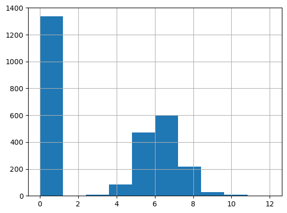

predictor = TabularPredictor(label='TargetSales_log1p').fit(train_df[selected_features+['TargetSales_log1p']],
                                                      presets=preset,
                                                      excluded_model_types=['NN_TORCH','FASTAI','KNN'],
                                                      )

No path specified. Models will be saved in: "AutogluonModels/ag-20241214_134958"
Verbosity: 2 (Standard Logging)
=================== System Info ===================
AutoGluon Version:  1.1.1
Python Version:     3.9.12
Operating System:   Linux
Platform Machine:   x86_64
Platform Version:   #1 SMP Wed Oct 23 01:22:11 UTC 2024
CPU Count:          64
Memory Avail:       468.19 GB / 480.23 GB (97.5%)
Disk Space Avail:   1451.46 GB / 1968.52 GB (73.7%)
===================================================
Presets specified: ['good_quality']
Setting dynamic_stacking from 'auto' to True. Reason: Enable dynamic_stacking when use_bag_holdout is disabled. (use_bag_holdout=False)
Stack configuration (auto_stack=True): num_stack_levels=1, num_bag_folds=8, num_bag_sets=1
Note: `save_bag_folds=False`! This will greatly reduce peak disk usage during fit (by ~8x), but runs the risk of an out-of-memory error during model refit if memory is small relative to the data size.
    You can avoid this risk by setting `save_bag_folds=True`.
DyStack is enabled (dynamic_stacking=True). AutoGluon will try to determine whether the input data is affected by stacked overfitting and enable or disable stacking as a consequence.
    This is used to identify the optimal `num_stack_levels` value. Copies of AutoGluon will be fit on subsets of the data. Then holdout validation data is used to detect stacked overfitting.
    Running DyStack for up to 900s of the 3600s of remaining time (25%).
/home/charipol/miniconda3/lib/python3.9/site-packages/autogluon/tabular/predictor/predictor.py:1242: UserWarning: Failed to use ray for memory safe fits. Falling back to normal fit. Error: ValueError('ray==2.40.0 detected. 2.10.0 <= ray < 2.11.0 is required. You can use pip to install certain version of ray `pip install ray==2.10.0` ')
  stacked_overfitting = self._sub_fit_memory_save_wrapper(
        Context path: "AutogluonModels/ag-20241214_134958/ds_sub_fit/sub_fit_ho"
Running DyStack sub-fit ...
Beginning AutoGluon training ... Time limit = 900s
AutoGluon will save models to "AutogluonModels/ag-20241214_134958/ds_sub_fit/sub_fit_ho"
Train Data Rows:    2444
Train Data Columns: 17
Label Column:       TargetSales_log1p
Problem Type:       regression
Preprocessing data ...
Using Feature Generators to preprocess the data ...
Fitting AutoMLPipelineFeatureGenerator...
    Available Memory:                    479431.23 MB
    Train Data (Original)  Memory Usage: 0.32 MB (0.0% of available memory)
    Inferring data type of each feature based on column values. Set feature_metadata_in to manually specify special dtypes of the features.
    Stage 1 Generators:
        Fitting AsTypeFeatureGenerator...
    Stage 2 Generators:
        Fitting FillNaFeatureGenerator...
    Stage 3 Generators:
        Fitting IdentityFeatureGenerator...
    Stage 4 Generators:
        Fitting DropUniqueFeatureGenerator...
    Stage 5 Generators:
        Fitting DropDuplicatesFeatureGenerator...
    Types of features in original data (raw dtype, special dtypes):
        ('float', []) : 12 | ['total_sales', 'avg_purchase_frequency', 'avg_purchase_value', 'per_fashion_accessories', 'per_home_decor', ...]
        ('int', [])   :  5 | ['recency', 'purchase_day', 'nb_product', 'nb_category', 'customer_lifetime']
    Types of features in processed data (raw dtype, special dtypes):
        ('float', []) : 12 | ['total_sales', 'avg_purchase_frequency', 'avg_purchase_value', 'per_fashion_accessories', 'per_home_decor', ...]
        ('int', [])   :  5 | ['recency', 'purchase_day', 'nb_product', 'nb_category', 'customer_lifetime']
    0.0s = Fit runtime
    17 features in original data used to generate 17 features in processed data.
    Train Data (Processed) Memory Usage: 0.32 MB (0.0% of available memory)
Data preprocessing and feature engineering runtime = 0.06s ...
AutoGluon will gauge predictive performance using evaluation metric: 'root_mean_squared_error'
    This metric's sign has been flipped to adhere to being higher_is_better. The metric score can be multiplied by -1 to get the metric value.
    To change this, specify the eval_metric parameter of Predictor()
User-specified model hyperparameters to be fit:
{
    'NN_TORCH': {},
    'GBM': [{'extra_trees': True, 'ag_args': {'name_suffix': 'XT'}}, {}, 'GBMLarge'],
    'CAT': {},
    'XGB': {},
    'FASTAI': {},
    'RF': [{'criterion': 'gini', 'max_depth': 15, 'ag_args': {'name_suffix': 'Gini', 'problem_types': ['binary', 'multiclass']}}, {'criterion': 'entropy', 'max_depth': 15, 'ag_args': {'name_suffix': 'Entr', 'problem_types': ['binary', 'multiclass']}}, {'criterion': 'squared_error', 'max_depth': 15, 'ag_args': {'name_suffix': 'MSE', 'problem_types': ['regression', 'quantile']}}],
    'XT': [{'criterion': 'gini', 'max_depth': 15, 'ag_args': {'name_suffix': 'Gini', 'problem_types': ['binary', 'multiclass']}}, {'criterion': 'entropy', 'max_depth': 15, 'ag_args': {'name_suffix': 'Entr', 'problem_types': ['binary', 'multiclass']}}, {'criterion': 'squared_error', 'max_depth': 15, 'ag_args': {'name_suffix': 'MSE', 'problem_types': ['regression', 'quantile']}}],
}
AutoGluon will fit 2 stack levels (L1 to L2) ...
Excluded models: ['NN_TORCH', 'FASTAI'] (Specified by `excluded_model_types`)
Fitting 7 L1 models ...
Fitting model: LightGBMXT_BAG_L1 ... Training model for up to 599.81s of the 899.94s of remaining time.
    Fitting 8 child models (S1F1 - S1F8) | Fitting with SequentialLocalFoldFittingStrategy
    -2.7823  = Validation score   (-root_mean_squared_error)
    4.54s    = Training   runtime
    0.01s    = Validation runtime
Fitting model: LightGBM_BAG_L1 ... Training model for up to 595.21s of the 895.34s of remaining time.
    Fitting 8 child models (S1F1 - S1F8) | Fitting with SequentialLocalFoldFittingStrategy
    -2.8135  = Validation score   (-root_mean_squared_error)
    3.9s     = Training   runtime
    0.01s    = Validation runtime
Fitting model: RandomForestMSE_BAG_L1 ... Training model for up to 591.22s of the 891.35s of remaining time.
    -2.8314  = Validation score   (-root_mean_squared_error)
    0.8s     = Training   runtime
    0.18s    = Validation runtime
Fitting model: CatBoost_BAG_L1 ... Training model for up to 590.14s of the 890.26s of remaining time.
    Fitting 8 child models (S1F1 - S1F8) | Fitting with SequentialLocalFoldFittingStrategy
    -2.7808  = Validation score   (-root_mean_squared_error)
    5.75s    = Training   runtime
    0.02s    = Validation runtime
Fitting model: ExtraTreesMSE_BAG_L1 ... Training model for up to 584.28s of the 884.41s of remaining time.
    -2.8158  = Validation score   (-root_mean_squared_error)
    0.68s    = Training   runtime
    0.18s    = Validation runtime
Fitting model: XGBoost_BAG_L1 ... Training model for up to 583.31s of the 883.44s of remaining time.
    Fitting 8 child models (S1F1 - S1F8) | Fitting with SequentialLocalFoldFittingStrategy
    -2.8362  = Validation score   (-root_mean_squared_error)
    5.3s     = Training   runtime
    0.03s    = Validation runtime
Fitting model: LightGBMLarge_BAG_L1 ... Training model for up to 577.92s of the 878.05s of remaining time.
    Fitting 8 child models (S1F1 - S1F8) | Fitting with SequentialLocalFoldFittingStrategy
    -2.8628  = Validation score   (-root_mean_squared_error)
    12.04s   = Training   runtime
    0.01s    = Validation runtime
Fitting model: WeightedEnsemble_L2 ... Training model for up to 360.0s of the 865.92s of remaining time.
    Ensemble Weights: {'CatBoost_BAG_L1': 0.478, 'LightGBMXT_BAG_L1': 0.435, 'ExtraTreesMSE_BAG_L1': 0.087}
    -2.7756  = Validation score   (-root_mean_squared_error)
    0.02s    = Training   runtime
    0.0s     = Validation runtime
Excluded models: ['NN_TORCH', 'FASTAI'] (Specified by `excluded_model_types`)
Fitting 7 L2 models ...
Fitting model: LightGBMXT_BAG_L2 ... Training model for up to 865.86s of the 865.85s of remaining time.
    Fitting 8 child models (S1F1 - S1F8) | Fitting with SequentialLocalFoldFittingStrategy

[1000]  valid_set's rmse: 2.69718
[2000]  valid_set's rmse: 2.65909
[3000]  valid_set's rmse: 2.65127
[4000]  valid_set's rmse: 2.64831
[5000]  valid_set's rmse: 2.64686
[6000]  valid_set's rmse: 2.64619
[7000]  valid_set's rmse: 2.64592
[8000]  valid_set's rmse: 2.64577
[9000]  valid_set's rmse: 2.64574
[10000] valid_set's rmse: 2.64573
[1000]  valid_set's rmse: 2.69753
[2000]  valid_set's rmse: 2.65357
[3000]  valid_set's rmse: 2.64919
[4000]  valid_set's rmse: 2.64645
[5000]  valid_set's rmse: 2.64479
[6000]  valid_set's rmse: 2.64422
[7000]  valid_set's rmse: 2.6439
[8000]  valid_set's rmse: 2.64387
[9000]  valid_set's rmse: 2.64384
[10000] valid_set's rmse: 2.64383
[1000]  valid_set's rmse: 2.71185
[2000]  valid_set's rmse: 2.66777
[3000]  valid_set's rmse: 2.65641
[4000]  valid_set's rmse: 2.65399
[5000]  valid_set's rmse: 2.65317
[6000]  valid_set's rmse: 2.65306
[7000]  valid_set's rmse: 2.65305
[1000]  valid_set's rmse: 2.73753
[2000]  valid_set's rmse: 2.69713
[3000]  valid_set's rmse: 2.68365
[4000]  valid_set's rmse: 2.67838
[5000]  valid_set's rmse: 2.67756
[6000]  valid_set's rmse: 2.67725
[7000]  valid_set's rmse: 2.67727
[1000]  valid_set's rmse: 2.51029
[2000]  valid_set's rmse: 2.46542
[3000]  valid_set's rmse: 2.45449
[4000]  valid_set's rmse: 2.45128
[5000]  valid_set's rmse: 2.44983
[6000]  valid_set's rmse: 2.44947
[7000]  valid_set's rmse: 2.44914
[8000]  valid_set's rmse: 2.44909
[9000]  valid_set's rmse: 2.4491
[10000] valid_set's rmse: 2.44914

    -2.6944  = Validation score   (-root_mean_squared_error)
    52.47s   = Training   runtime
    0.08s    = Validation runtime
Fitting model: LightGBM_BAG_L2 ... Training model for up to 813.19s of the 813.18s of remaining time.
    Fitting 8 child models (S1F1 - S1F8) | Fitting with SequentialLocalFoldFittingStrategy

[1000]  valid_set's rmse: 2.64699
[2000]  valid_set's rmse: 2.64384
[3000]  valid_set's rmse: 2.64347
[4000]  valid_set's rmse: 2.64345
[1000]  valid_set's rmse: 2.6483
[1000]  valid_set's rmse: 2.87823

    -2.7598  = Validation score   (-root_mean_squared_error)
    9.99s    = Training   runtime
    0.02s    = Validation runtime
Fitting model: RandomForestMSE_BAG_L2 ... Training model for up to 803.1s of the 803.09s of remaining time.
    -2.8088  = Validation score   (-root_mean_squared_error)
    0.75s    = Training   runtime
    0.18s    = Validation runtime
Fitting model: CatBoost_BAG_L2 ... Training model for up to 802.07s of the 802.06s of remaining time.
    Fitting 8 child models (S1F1 - S1F8) | Fitting with SequentialLocalFoldFittingStrategy
    -2.759   = Validation score   (-root_mean_squared_error)
    92.85s   = Training   runtime
    0.04s    = Validation runtime
Fitting model: ExtraTreesMSE_BAG_L2 ... Training model for up to 709.08s of the 709.07s of remaining time.
    -2.778   = Validation score   (-root_mean_squared_error)
    0.66s    = Training   runtime
    0.18s    = Validation runtime
Fitting model: XGBoost_BAG_L2 ... Training model for up to 708.14s of the 708.13s of remaining time.
    Fitting 8 child models (S1F1 - S1F8) | Fitting with SequentialLocalFoldFittingStrategy
    -2.7901  = Validation score   (-root_mean_squared_error)
    6.46s    = Training   runtime
    0.03s    = Validation runtime
Fitting model: LightGBMLarge_BAG_L2 ... Training model for up to 701.58s of the 701.57s of remaining time.
    Fitting 8 child models (S1F1 - S1F8) | Fitting with SequentialLocalFoldFittingStrategy

[1000]  valid_set's rmse: 2.76447
[1000]  valid_set's rmse: 2.80146
[2000]  valid_set's rmse: 2.8014
[3000]  valid_set's rmse: 2.8014
[4000]  valid_set's rmse: 2.8014
[1000]  valid_set's rmse: 2.88446
[2000]  valid_set's rmse: 2.88439

    -2.7943  = Validation score   (-root_mean_squared_error)
    45.94s   = Training   runtime
    0.04s    = Validation runtime
Fitting model: WeightedEnsemble_L3 ... Training model for up to 360.0s of the 655.49s of remaining time.
    Ensemble Weights: {'LightGBMXT_BAG_L2': 0.72, 'CatBoost_BAG_L1': 0.12, 'LightGBMXT_BAG_L1': 0.04, 'LightGBM_BAG_L2': 0.04, 'XGBoost_BAG_L2': 0.04, 'LightGBMLarge_BAG_L2': 0.04}
    -2.6854  = Validation score   (-root_mean_squared_error)
    0.03s    = Training   runtime
    0.0s     = Validation runtime
AutoGluon training complete, total runtime = 244.6s ... Best model: WeightedEnsemble_L3 | Estimated inference throughput: 1078.2 rows/s (306 batch size)
Automatically performing refit_full as a post-fit operation (due to `.fit(..., refit_full=True)`
Refitting models via `predictor.refit_full` using all of the data (combined train and validation)...
    Models trained in this way will have the suffix "_FULL" and have NaN validation score.
    This process is not bound by time_limit, but should take less time than the original `predictor.fit` call.
    To learn more, refer to the `.refit_full` method docstring which explains how "_FULL" models differ from normal models.
Fitting 1 L1 models ...
Fitting model: LightGBMXT_BAG_L1_FULL ...
    0.23s    = Training   runtime
Fitting 1 L1 models ...
Fitting model: LightGBM_BAG_L1_FULL ...
    0.17s    = Training   runtime
Fitting model: RandomForestMSE_BAG_L1_FULL | Skipping fit via cloning parent ...
    0.8s     = Training   runtime
    0.18s    = Validation runtime
Fitting 1 L1 models ...
Fitting model: CatBoost_BAG_L1_FULL ...
    0.21s    = Training   runtime
Fitting model: ExtraTreesMSE_BAG_L1_FULL | Skipping fit via cloning parent ...
    0.68s    = Training   runtime
    0.18s    = Validation runtime
Fitting 1 L1 models ...
Fitting model: XGBoost_BAG_L1_FULL ...
    0.08s    = Training   runtime
Fitting 1 L1 models ...
Fitting model: LightGBMLarge_BAG_L1_FULL ...
    0.37s    = Training   runtime
Fitting model: WeightedEnsemble_L2_FULL | Skipping fit via cloning parent ...
    Ensemble Weights: {'CatBoost_BAG_L1': 0.478, 'LightGBMXT_BAG_L1': 0.435, 'ExtraTreesMSE_BAG_L1': 0.087}
    0.02s    = Training   runtime
Fitting 1 L2 models ...
Fitting model: LightGBMXT_BAG_L2_FULL ...
    4.94s    = Training   runtime
Fitting 1 L2 models ...
Fitting model: LightGBM_BAG_L2_FULL ...
    0.76s    = Training   runtime
Fitting model: RandomForestMSE_BAG_L2_FULL | Skipping fit via cloning parent ...
    0.75s    = Training   runtime
    0.18s    = Validation runtime
Fitting 1 L2 models ...
Fitting model: CatBoost_BAG_L2_FULL ...
    3.03s    = Training   runtime
Fitting model: ExtraTreesMSE_BAG_L2_FULL | Skipping fit via cloning parent ...
    0.66s    = Training   runtime
    0.18s    = Validation runtime
Fitting 1 L2 models ...
Fitting model: XGBoost_BAG_L2_FULL ...
    0.16s    = Training   runtime
Fitting 1 L2 models ...
Fitting model: LightGBMLarge_BAG_L2_FULL ...
    3.93s    = Training   runtime
Fitting model: WeightedEnsemble_L3_FULL | Skipping fit via cloning parent ...
    Ensemble Weights: {'LightGBMXT_BAG_L2': 0.72, 'CatBoost_BAG_L1': 0.12, 'LightGBMXT_BAG_L1': 0.04, 'LightGBM_BAG_L2': 0.04, 'XGBoost_BAG_L2': 0.04, 'LightGBMLarge_BAG_L2': 0.04}
    0.03s    = Training   runtime
Updated best model to "WeightedEnsemble_L3_FULL" (Previously "WeightedEnsemble_L3"). AutoGluon will default to using "WeightedEnsemble_L3_FULL" for predict() and predict_proba().
Refit complete, total runtime = 14.81s ... Best model: "WeightedEnsemble_L3_FULL"
TabularPredictor saved. To load, use: predictor = TabularPredictor.load("AutogluonModels/ag-20241214_134958/ds_sub_fit/sub_fit_ho")
Deleting DyStack predictor artifacts (clean_up_fits=True) ...
Leaderboard on holdout data (DyStack):
                          model  score_holdout  score_val              eval_metric  pred_time_test  pred_time_val   fit_time  pred_time_test_marginal  pred_time_val_marginal  fit_time_marginal  stack_level  can_infer  fit_order
0          CatBoost_BAG_L1_FULL      -2.885523  -2.780750  root_mean_squared_error        0.019700            NaN   0.210621                 0.019700                     NaN           0.210621            1       True          4
1      WeightedEnsemble_L2_FULL      -2.894191  -2.775644  root_mean_squared_error        0.155056            NaN   1.140924                 0.002549                     NaN           0.019073            2       True          8
2   RandomForestMSE_BAG_L2_FULL      -2.894937  -2.808770  root_mean_squared_error        0.407366            NaN   3.299085                 0.126307                0.179813           0.754930            2       True         11
3     ExtraTreesMSE_BAG_L2_FULL      -2.896741  -2.777983  root_mean_squared_error        0.400050            NaN   3.203568                 0.118991                0.182625           0.659413            2       True         13
4        LightGBMXT_BAG_L1_FULL      -2.908863  -2.782297  root_mean_squared_error        0.002410            NaN   0.229015                 0.002410                     NaN           0.229015            1       True          1
5          CatBoost_BAG_L2_FULL      -2.922107  -2.759026  root_mean_squared_error        0.290997            NaN   5.576536                 0.009938                     NaN           3.032381            2       True         12
6          LightGBM_BAG_L2_FULL      -2.931031  -2.759814  root_mean_squared_error        0.291885            NaN   3.309105                 0.010826                     NaN           0.764950            2       True         10
7           XGBoost_BAG_L2_FULL      -2.938193  -2.790059  root_mean_squared_error        0.292573            NaN   2.701340                 0.011514                     NaN           0.157185            2       True         14
8      WeightedEnsemble_L3_FULL      -2.942265  -2.685363  root_mean_squared_error        0.414771            NaN  12.371993                 0.005430                     NaN           0.029768            3       True         16
9     ExtraTreesMSE_BAG_L1_FULL      -2.946022  -2.815757  root_mean_squared_error        0.130396       0.183574   0.682215                 0.130396                0.183574           0.682215            1       True          5
10         LightGBM_BAG_L1_FULL      -2.953480  -2.813496  root_mean_squared_error        0.001765            NaN   0.174514                 0.001765                     NaN           0.174514            1       True          2
11          XGBoost_BAG_L1_FULL      -2.972277  -2.836214  root_mean_squared_error        0.010018            NaN   0.076469                 0.010018                     NaN           0.076469            1       True          6
12    LightGBMLarge_BAG_L2_FULL      -2.977587  -2.794323  root_mean_squared_error        0.327995            NaN   6.475816                 0.046936                     NaN           3.931662            2       True         15
13  RandomForestMSE_BAG_L1_FULL      -2.985264  -2.831375  root_mean_squared_error        0.111768       0.181522   0.798739                 0.111768                0.181522           0.798739            1       True          3
14       LightGBMXT_BAG_L2_FULL      -2.995407  -2.694352  root_mean_squared_error        0.340065            NaN   7.488428                 0.059006                     NaN           4.944273            2       True          9
15    LightGBMLarge_BAG_L1_FULL      -3.050660  -2.862792  root_mean_squared_error        0.005002            NaN   0.372581                 0.005002                     NaN           0.372581            1       True          7
    0    = Optimal   num_stack_levels (Stacked Overfitting Occurred: True)
    260s     = DyStack   runtime |  3340s    = Remaining runtime
Starting main fit with num_stack_levels=0.
    For future fit calls on this dataset, you can skip DyStack to save time: `predictor.fit(..., dynamic_stacking=False, num_stack_levels=0)`
Beginning AutoGluon training ... Time limit = 3340s
AutoGluon will save models to "AutogluonModels/ag-20241214_134958"
Train Data Rows:    2750
Train Data Columns: 17
Label Column:       TargetSales_log1p
Problem Type:       regression
Preprocessing data ...
Using Feature Generators to preprocess the data ...
Fitting AutoMLPipelineFeatureGenerator...
    Available Memory:                    479126.25 MB
    Train Data (Original)  Memory Usage: 0.36 MB (0.0% of available memory)
    Inferring data type of each feature based on column values. Set feature_metadata_in to manually specify special dtypes of the features.
    Stage 1 Generators:
        Fitting AsTypeFeatureGenerator...
    Stage 2 Generators:
        Fitting FillNaFeatureGenerator...
    Stage 3 Generators:
        Fitting IdentityFeatureGenerator...
    Stage 4 Generators:
        Fitting DropUniqueFeatureGenerator...
    Stage 5 Generators:
        Fitting DropDuplicatesFeatureGenerator...
    Types of features in original data (raw dtype, special dtypes):
        ('float', []) : 12 | ['total_sales', 'avg_purchase_frequency', 'avg_purchase_value', 'per_fashion_accessories', 'per_home_decor', ...]
        ('int', [])   :  5 | ['recency', 'purchase_day', 'nb_product', 'nb_category', 'customer_lifetime']
    Types of features in processed data (raw dtype, special dtypes):
        ('float', []) : 12 | ['total_sales', 'avg_purchase_frequency', 'avg_purchase_value', 'per_fashion_accessories', 'per_home_decor', ...]
        ('int', [])   :  5 | ['recency', 'purchase_day', 'nb_product', 'nb_category', 'customer_lifetime']
    0.0s = Fit runtime
    17 features in original data used to generate 17 features in processed data.
    Train Data (Processed) Memory Usage: 0.36 MB (0.0% of available memory)
Data preprocessing and feature engineering runtime = 0.07s ...
AutoGluon will gauge predictive performance using evaluation metric: 'root_mean_squared_error'
    This metric's sign has been flipped to adhere to being higher_is_better. The metric score can be multiplied by -1 to get the metric value.
    To change this, specify the eval_metric parameter of Predictor()
User-specified model hyperparameters to be fit:
{
    'NN_TORCH': {},
    'GBM': [{'extra_trees': True, 'ag_args': {'name_suffix': 'XT'}}, {}, 'GBMLarge'],
    'CAT': {},
    'XGB': {},
    'FASTAI': {},
    'RF': [{'criterion': 'gini', 'max_depth': 15, 'ag_args': {'name_suffix': 'Gini', 'problem_types': ['binary', 'multiclass']}}, {'criterion': 'entropy', 'max_depth': 15, 'ag_args': {'name_suffix': 'Entr', 'problem_types': ['binary', 'multiclass']}}, {'criterion': 'squared_error', 'max_depth': 15, 'ag_args': {'name_suffix': 'MSE', 'problem_types': ['regression', 'quantile']}}],
    'XT': [{'criterion': 'gini', 'max_depth': 15, 'ag_args': {'name_suffix': 'Gini', 'problem_types': ['binary', 'multiclass']}}, {'criterion': 'entropy', 'max_depth': 15, 'ag_args': {'name_suffix': 'Entr', 'problem_types': ['binary', 'multiclass']}}, {'criterion': 'squared_error', 'max_depth': 15, 'ag_args': {'name_suffix': 'MSE', 'problem_types': ['regression', 'quantile']}}],
}
Excluded models: ['NN_TORCH', 'FASTAI'] (Specified by `excluded_model_types`)
Fitting 7 L1 models ...
Fitting model: LightGBMXT_BAG_L1 ... Training model for up to 3339.69s of the 3339.68s of remaining time.
    Fitting 8 child models (S1F1 - S1F8) | Fitting with SequentialLocalFoldFittingStrategy
    -2.7861  = Validation score   (-root_mean_squared_error)
    5.11s    = Training   runtime
    0.01s    = Validation runtime
Fitting model: LightGBM_BAG_L1 ... Training model for up to 3334.48s of the 3334.48s of remaining time.
    Fitting 8 child models (S1F1 - S1F8) | Fitting with SequentialLocalFoldFittingStrategy
    -2.8189  = Validation score   (-root_mean_squared_error)
    4.72s    = Training   runtime
    0.01s    = Validation runtime
Fitting model: RandomForestMSE_BAG_L1 ... Training model for up to 3329.67s of the 3329.67s of remaining time.
    -2.8468  = Validation score   (-root_mean_squared_error)
    0.72s    = Training   runtime
    0.19s    = Validation runtime
Fitting model: CatBoost_BAG_L1 ... Training model for up to 3328.66s of the 3328.66s of remaining time.
    Fitting 8 child models (S1F1 - S1F8) | Fitting with SequentialLocalFoldFittingStrategy
    -2.7963  = Validation score   (-root_mean_squared_error)
    5.43s    = Training   runtime
    0.02s    = Validation runtime
Fitting model: ExtraTreesMSE_BAG_L1 ... Training model for up to 3323.13s of the 3323.13s of remaining time.
    -2.8191  = Validation score   (-root_mean_squared_error)
    0.66s    = Training   runtime
    0.19s    = Validation runtime
Fitting model: XGBoost_BAG_L1 ... Training model for up to 3322.18s of the 3322.18s of remaining time.
    Fitting 8 child models (S1F1 - S1F8) | Fitting with SequentialLocalFoldFittingStrategy
    -2.8365  = Validation score   (-root_mean_squared_error)
    5.51s    = Training   runtime
    0.04s    = Validation runtime
Fitting model: LightGBMLarge_BAG_L1 ... Training model for up to 3316.57s of the 3316.57s of remaining time.
    Fitting 8 child models (S1F1 - S1F8) | Fitting with SequentialLocalFoldFittingStrategy
    -2.8667  = Validation score   (-root_mean_squared_error)
    12.3s    = Training   runtime
    0.01s    = Validation runtime
Fitting model: WeightedEnsemble_L2 ... Training model for up to 360.0s of the 3304.17s of remaining time.
    Ensemble Weights: {'LightGBMXT_BAG_L1': 0.714, 'CatBoost_BAG_L1': 0.143, 'ExtraTreesMSE_BAG_L1': 0.143}
    -2.7845  = Validation score   (-root_mean_squared_error)
    0.02s    = Training   runtime
    0.0s     = Validation runtime
AutoGluon training complete, total runtime = 35.65s ... Best model: WeightedEnsemble_L2 | Estimated inference throughput: 6632.0 rows/s (344 batch size)
Automatically performing refit_full as a post-fit operation (due to `.fit(..., refit_full=True)`
Refitting models via `predictor.refit_full` using all of the data (combined train and validation)...
    Models trained in this way will have the suffix "_FULL" and have NaN validation score.
    This process is not bound by time_limit, but should take less time than the original `predictor.fit` call.
    To learn more, refer to the `.refit_full` method docstring which explains how "_FULL" models differ from normal models.
Fitting 1 L1 models ...
Fitting model: LightGBMXT_BAG_L1_FULL ...
    0.21s    = Training   runtime
Fitting 1 L1 models ...
Fitting model: LightGBM_BAG_L1_FULL ...
    0.19s    = Training   runtime
Fitting model: RandomForestMSE_BAG_L1_FULL | Skipping fit via cloning parent ...
    0.72s    = Training   runtime
    0.19s    = Validation runtime
Fitting 1 L1 models ...
Fitting model: CatBoost_BAG_L1_FULL ...
    0.18s    = Training   runtime
Fitting model: ExtraTreesMSE_BAG_L1_FULL | Skipping fit via cloning parent ...
    0.66s    = Training   runtime
    0.19s    = Validation runtime
Fitting 1 L1 models ...
Fitting model: XGBoost_BAG_L1_FULL ...
    0.09s    = Training   runtime
Fitting 1 L1 models ...
Fitting model: LightGBMLarge_BAG_L1_FULL ...
    0.41s    = Training   runtime
Fitting model: WeightedEnsemble_L2_FULL | Skipping fit via cloning parent ...
    Ensemble Weights: {'LightGBMXT_BAG_L1': 0.714, 'CatBoost_BAG_L1': 0.143, 'ExtraTreesMSE_BAG_L1': 0.143}
    0.02s    = Training   runtime
Updated best model to "WeightedEnsemble_L2_FULL" (Previously "WeightedEnsemble_L2"). AutoGluon will default to using "WeightedEnsemble_L2_FULL" for predict() and predict_proba().
Refit complete, total runtime = 1.41s ... Best model: "WeightedEnsemble_L2_FULL"
TabularPredictor saved. To load, use: predictor = TabularPredictor.load("AutogluonModels/ag-20241214_134958")

test_df['pred_log1p'] = predictor.predict(test_df[selected_features])
test_df['pred_log1p_expm1'] = test_df['pred_log1p'].map(np.expm1)

metric_log1p = calculate_regression_metrics(test_df['TargetSales'], test_df['pred_log1p_expm1'])
metric_log1p['model'] = 'log1p'
metric_log1p

{'root_mean_squared_error': 3725.342295894091,
 'mean_squared_error': 13878175.221577456,
 'mean_absolute_error': 618.9768466651894,
 'r2': 0.14190585634701047,
 'pearsonr': 0.5817166874396966,
 'spearmanr': 0.5338156315937898,
 'median_absolute_error': 89.55495441784018,
 'earths_mover_distance': 581.0494444960044,
 'model': 'log1p'}

calculate_regression_metrics(test_df['TargetSales_log1p'], test_df['pred_log1p'])

{'root_mean_squared_error': 2.720047847858299,
 'mean_squared_error': 7.398660294638562,
 'mean_absolute_error': 2.418601533469381,
 'r2': 0.30252750020590236,
 'pearsonr': 0.5507740732825224,
 'spearmanr': 0.5338156315937898,
 'median_absolute_error': 2.349368453025818,
 'earths_mover_distance': 1.8552344547363062}

Hurdle Model

Hurdle model is a two-stage approach that handles zero inflation by first having a classification model to predict if the outcome is zero or not, then a regression model, trained only on examples with actual non-zero outcomes, to fit a log-transformed outcome. When retransforming the predictions from log to non-log numbers, we perform correction of underestimation using Duan’s method. During inference time, we multiply the predictions from the classification and regression model.

Binary Classification

train_df['has_purchase'] = train_df.TargetSales.map(lambda x: 1 if x>0 else 0)
test_df['has_purchase'] = test_df.TargetSales.map(lambda x: 1 if x>0 else 0)

train_df['has_purchase'].mean(), test_df['has_purchase'].mean()

(0.5141818181818182, 0.5305232558139535)

predictor_cls = TabularPredictor(label='has_purchase').fit(train_df[selected_features+['has_purchase']],
                                                      presets=preset,
                                                      excluded_model_types=['NN_TORCH','FASTAI','KNN'],
                                                      )

No path specified. Models will be saved in: "AutogluonModels/ag-20241214_135456"
Verbosity: 2 (Standard Logging)
=================== System Info ===================
AutoGluon Version:  1.1.1
Python Version:     3.9.12
Operating System:   Linux
Platform Machine:   x86_64
Platform Version:   #1 SMP Wed Oct 23 01:22:11 UTC 2024
CPU Count:          64
Memory Avail:       467.88 GB / 480.23 GB (97.4%)
Disk Space Avail:   1451.34 GB / 1968.52 GB (73.7%)
===================================================
Presets specified: ['good_quality']
Setting dynamic_stacking from 'auto' to True. Reason: Enable dynamic_stacking when use_bag_holdout is disabled. (use_bag_holdout=False)
Stack configuration (auto_stack=True): num_stack_levels=1, num_bag_folds=8, num_bag_sets=1
Note: `save_bag_folds=False`! This will greatly reduce peak disk usage during fit (by ~8x), but runs the risk of an out-of-memory error during model refit if memory is small relative to the data size.
    You can avoid this risk by setting `save_bag_folds=True`.
DyStack is enabled (dynamic_stacking=True). AutoGluon will try to determine whether the input data is affected by stacked overfitting and enable or disable stacking as a consequence.
    This is used to identify the optimal `num_stack_levels` value. Copies of AutoGluon will be fit on subsets of the data. Then holdout validation data is used to detect stacked overfitting.
    Running DyStack for up to 900s of the 3600s of remaining time (25%).
/home/charipol/miniconda3/lib/python3.9/site-packages/autogluon/tabular/predictor/predictor.py:1242: UserWarning: Failed to use ray for memory safe fits. Falling back to normal fit. Error: ValueError('ray==2.40.0 detected. 2.10.0 <= ray < 2.11.0 is required. You can use pip to install certain version of ray `pip install ray==2.10.0` ')
  stacked_overfitting = self._sub_fit_memory_save_wrapper(
        Context path: "AutogluonModels/ag-20241214_135456/ds_sub_fit/sub_fit_ho"
Running DyStack sub-fit ...
Beginning AutoGluon training ... Time limit = 900s
AutoGluon will save models to "AutogluonModels/ag-20241214_135456/ds_sub_fit/sub_fit_ho"
Train Data Rows:    2444
Train Data Columns: 17
Label Column:       has_purchase
Problem Type:       binary
Preprocessing data ...
Selected class <--> label mapping:  class 1 = 1, class 0 = 0
Using Feature Generators to preprocess the data ...
Fitting AutoMLPipelineFeatureGenerator...
    Available Memory:                    479111.52 MB
    Train Data (Original)  Memory Usage: 0.32 MB (0.0% of available memory)
    Inferring data type of each feature based on column values. Set feature_metadata_in to manually specify special dtypes of the features.
    Stage 1 Generators:
        Fitting AsTypeFeatureGenerator...
    Stage 2 Generators:
        Fitting FillNaFeatureGenerator...
    Stage 3 Generators:
        Fitting IdentityFeatureGenerator...
    Stage 4 Generators:
        Fitting DropUniqueFeatureGenerator...
    Stage 5 Generators:
        Fitting DropDuplicatesFeatureGenerator...
    Types of features in original data (raw dtype, special dtypes):
        ('float', []) : 12 | ['total_sales', 'avg_purchase_frequency', 'avg_purchase_value', 'per_fashion_accessories', 'per_home_decor', ...]
        ('int', [])   :  5 | ['recency', 'purchase_day', 'nb_product', 'nb_category', 'customer_lifetime']
    Types of features in processed data (raw dtype, special dtypes):
        ('float', []) : 12 | ['total_sales', 'avg_purchase_frequency', 'avg_purchase_value', 'per_fashion_accessories', 'per_home_decor', ...]
        ('int', [])   :  5 | ['recency', 'purchase_day', 'nb_product', 'nb_category', 'customer_lifetime']
    0.1s = Fit runtime
    17 features in original data used to generate 17 features in processed data.
    Train Data (Processed) Memory Usage: 0.32 MB (0.0% of available memory)
Data preprocessing and feature engineering runtime = 0.08s ...
AutoGluon will gauge predictive performance using evaluation metric: 'accuracy'
    To change this, specify the eval_metric parameter of Predictor()
User-specified model hyperparameters to be fit:
{
    'NN_TORCH': {},
    'GBM': [{'extra_trees': True, 'ag_args': {'name_suffix': 'XT'}}, {}, 'GBMLarge'],
    'CAT': {},
    'XGB': {},
    'FASTAI': {},
    'RF': [{'criterion': 'gini', 'max_depth': 15, 'ag_args': {'name_suffix': 'Gini', 'problem_types': ['binary', 'multiclass']}}, {'criterion': 'entropy', 'max_depth': 15, 'ag_args': {'name_suffix': 'Entr', 'problem_types': ['binary', 'multiclass']}}, {'criterion': 'squared_error', 'max_depth': 15, 'ag_args': {'name_suffix': 'MSE', 'problem_types': ['regression', 'quantile']}}],
    'XT': [{'criterion': 'gini', 'max_depth': 15, 'ag_args': {'name_suffix': 'Gini', 'problem_types': ['binary', 'multiclass']}}, {'criterion': 'entropy', 'max_depth': 15, 'ag_args': {'name_suffix': 'Entr', 'problem_types': ['binary', 'multiclass']}}, {'criterion': 'squared_error', 'max_depth': 15, 'ag_args': {'name_suffix': 'MSE', 'problem_types': ['regression', 'quantile']}}],
}
AutoGluon will fit 2 stack levels (L1 to L2) ...
Excluded models: ['NN_TORCH', 'FASTAI'] (Specified by `excluded_model_types`)
Fitting 9 L1 models ...
Fitting model: LightGBMXT_BAG_L1 ... Training model for up to 599.8s of the 899.92s of remaining time.
    Fitting 8 child models (S1F1 - S1F8) | Fitting with SequentialLocalFoldFittingStrategy
    0.6944   = Validation score   (accuracy)
    4.76s    = Training   runtime
    0.01s    = Validation runtime
Fitting model: LightGBM_BAG_L1 ... Training model for up to 594.97s of the 895.09s of remaining time.
    Fitting 8 child models (S1F1 - S1F8) | Fitting with SequentialLocalFoldFittingStrategy
    0.687    = Validation score   (accuracy)
    4.01s    = Training   runtime
    0.01s    = Validation runtime
Fitting model: RandomForestGini_BAG_L1 ... Training model for up to 590.87s of the 890.99s of remaining time.
    0.6661   = Validation score   (accuracy)
    0.88s    = Training   runtime
    0.18s    = Validation runtime
Fitting model: RandomForestEntr_BAG_L1 ... Training model for up to 589.72s of the 889.84s of remaining time.
    0.6543   = Validation score   (accuracy)
    0.88s    = Training   runtime
    0.18s    = Validation runtime
Fitting model: CatBoost_BAG_L1 ... Training model for up to 588.58s of the 888.7s of remaining time.
    Fitting 8 child models (S1F1 - S1F8) | Fitting with SequentialLocalFoldFittingStrategy
    0.698    = Validation score   (accuracy)
    8.46s    = Training   runtime
    0.02s    = Validation runtime
Fitting model: ExtraTreesGini_BAG_L1 ... Training model for up to 580.02s of the 880.14s of remaining time.
    0.6731   = Validation score   (accuracy)
    0.85s    = Training   runtime
    0.18s    = Validation runtime
Fitting model: ExtraTreesEntr_BAG_L1 ... Training model for up to 578.92s of the 879.04s of remaining time.
    0.6751   = Validation score   (accuracy)
    0.83s    = Training   runtime
    0.19s    = Validation runtime
Fitting model: XGBoost_BAG_L1 ... Training model for up to 577.82s of the 877.94s of remaining time.
    Fitting 8 child models (S1F1 - S1F8) | Fitting with SequentialLocalFoldFittingStrategy
    0.6874   = Validation score   (accuracy)
    4.94s    = Training   runtime
    0.03s    = Validation runtime
Fitting model: LightGBMLarge_BAG_L1 ... Training model for up to 572.75s of the 872.87s of remaining time.
    Fitting 8 child models (S1F1 - S1F8) | Fitting with SequentialLocalFoldFittingStrategy
    0.6739   = Validation score   (accuracy)
    16.57s   = Training   runtime
    0.01s    = Validation runtime
Fitting model: WeightedEnsemble_L2 ... Training model for up to 360.0s of the 856.19s of remaining time.
    Ensemble Weights: {'CatBoost_BAG_L1': 1.0}
    0.698    = Validation score   (accuracy)
    0.17s    = Training   runtime
    0.0s     = Validation runtime
Excluded models: ['NN_TORCH', 'FASTAI'] (Specified by `excluded_model_types`)
Fitting 9 L2 models ...
Fitting model: LightGBMXT_BAG_L2 ... Training model for up to 855.98s of the 855.97s of remaining time.
    Fitting 8 child models (S1F1 - S1F8) | Fitting with SequentialLocalFoldFittingStrategy
    0.7017   = Validation score   (accuracy)
    4.74s    = Training   runtime
    0.01s    = Validation runtime
Fitting model: LightGBM_BAG_L2 ... Training model for up to 851.17s of the 851.16s of remaining time.
    Fitting 8 child models (S1F1 - S1F8) | Fitting with SequentialLocalFoldFittingStrategy
    0.7062   = Validation score   (accuracy)
    4.62s    = Training   runtime
    0.01s    = Validation runtime
Fitting model: RandomForestGini_BAG_L2 ... Training model for up to 846.46s of the 846.45s of remaining time.
    0.6849   = Validation score   (accuracy)
    0.86s    = Training   runtime
    0.18s    = Validation runtime
Fitting model: RandomForestEntr_BAG_L2 ... Training model for up to 845.32s of the 845.31s of remaining time.
    0.6845   = Validation score   (accuracy)
    0.9s     = Training   runtime
    0.18s    = Validation runtime
Fitting model: CatBoost_BAG_L2 ... Training model for up to 844.16s of the 844.15s of remaining time.
    Fitting 8 child models (S1F1 - S1F8) | Fitting with SequentialLocalFoldFittingStrategy
    0.7074   = Validation score   (accuracy)
    12.05s   = Training   runtime
    0.02s    = Validation runtime
Fitting model: ExtraTreesGini_BAG_L2 ... Training model for up to 831.99s of the 831.98s of remaining time.
    0.6845   = Validation score   (accuracy)
    0.84s    = Training   runtime
    0.19s    = Validation runtime
Fitting model: ExtraTreesEntr_BAG_L2 ... Training model for up to 830.87s of the 830.86s of remaining time.
    0.6796   = Validation score   (accuracy)
    0.81s    = Training   runtime
    0.18s    = Validation runtime
Fitting model: XGBoost_BAG_L2 ... Training model for up to 829.78s of the 829.77s of remaining time.
    Fitting 8 child models (S1F1 - S1F8) | Fitting with SequentialLocalFoldFittingStrategy
    0.7029   = Validation score   (accuracy)
    5.77s    = Training   runtime
    0.03s    = Validation runtime
Fitting model: LightGBMLarge_BAG_L2 ... Training model for up to 823.88s of the 823.87s of remaining time.
    Fitting 8 child models (S1F1 - S1F8) | Fitting with SequentialLocalFoldFittingStrategy
    0.705    = Validation score   (accuracy)
    17.18s   = Training   runtime
    0.01s    = Validation runtime
Fitting model: WeightedEnsemble_L3 ... Training model for up to 360.0s of the 806.57s of remaining time.
    Ensemble Weights: {'CatBoost_BAG_L2': 0.957, 'CatBoost_BAG_L1': 0.043}
    0.7079   = Validation score   (accuracy)
    0.34s    = Training   runtime
    0.0s     = Validation runtime
AutoGluon training complete, total runtime = 93.82s ... Best model: WeightedEnsemble_L3 | Estimated inference throughput: 1613.2 rows/s (306 batch size)
Automatically performing refit_full as a post-fit operation (due to `.fit(..., refit_full=True)`
Refitting models via `predictor.refit_full` using all of the data (combined train and validation)...
    Models trained in this way will have the suffix "_FULL" and have NaN validation score.
    This process is not bound by time_limit, but should take less time than the original `predictor.fit` call.
    To learn more, refer to the `.refit_full` method docstring which explains how "_FULL" models differ from normal models.
Fitting 1 L1 models ...
Fitting model: LightGBMXT_BAG_L1_FULL ...
    0.27s    = Training   runtime
Fitting 1 L1 models ...
Fitting model: LightGBM_BAG_L1_FULL ...
    0.21s    = Training   runtime
Fitting model: RandomForestGini_BAG_L1_FULL | Skipping fit via cloning parent ...
    0.88s    = Training   runtime
    0.18s    = Validation runtime
Fitting model: RandomForestEntr_BAG_L1_FULL | Skipping fit via cloning parent ...
    0.88s    = Training   runtime
    0.18s    = Validation runtime
Fitting 1 L1 models ...
Fitting model: CatBoost_BAG_L1_FULL ...
    0.17s    = Training   runtime
Fitting model: ExtraTreesGini_BAG_L1_FULL | Skipping fit via cloning parent ...
    0.85s    = Training   runtime
    0.18s    = Validation runtime
Fitting model: ExtraTreesEntr_BAG_L1_FULL | Skipping fit via cloning parent ...
    0.83s    = Training   runtime
    0.19s    = Validation runtime
Fitting 1 L1 models ...
Fitting model: XGBoost_BAG_L1_FULL ...
    0.1s     = Training   runtime
Fitting 1 L1 models ...
Fitting model: LightGBMLarge_BAG_L1_FULL ...
    0.93s    = Training   runtime
Fitting model: WeightedEnsemble_L2_FULL | Skipping fit via cloning parent ...
    Ensemble Weights: {'CatBoost_BAG_L1': 1.0}
    0.17s    = Training   runtime
Fitting 1 L2 models ...
Fitting model: LightGBMXT_BAG_L2_FULL ...
    0.23s    = Training   runtime
Fitting 1 L2 models ...
Fitting model: LightGBM_BAG_L2_FULL ...
    0.23s    = Training   runtime
Fitting model: RandomForestGini_BAG_L2_FULL | Skipping fit via cloning parent ...
    0.86s    = Training   runtime
    0.18s    = Validation runtime
Fitting model: RandomForestEntr_BAG_L2_FULL | Skipping fit via cloning parent ...
    0.9s     = Training   runtime
    0.18s    = Validation runtime
Fitting 1 L2 models ...
Fitting model: CatBoost_BAG_L2_FULL ...
    0.58s    = Training   runtime
Fitting model: ExtraTreesGini_BAG_L2_FULL | Skipping fit via cloning parent ...
    0.84s    = Training   runtime
    0.19s    = Validation runtime
Fitting model: ExtraTreesEntr_BAG_L2_FULL | Skipping fit via cloning parent ...
    0.81s    = Training   runtime
    0.18s    = Validation runtime
Fitting 1 L2 models ...
Fitting model: XGBoost_BAG_L2_FULL ...
    0.12s    = Training   runtime
Fitting 1 L2 models ...
Fitting model: LightGBMLarge_BAG_L2_FULL ...
    0.89s    = Training   runtime
Fitting model: WeightedEnsemble_L3_FULL | Skipping fit via cloning parent ...
    Ensemble Weights: {'CatBoost_BAG_L2': 0.957, 'CatBoost_BAG_L1': 0.043}
    0.34s    = Training   runtime
Updated best model to "WeightedEnsemble_L3_FULL" (Previously "WeightedEnsemble_L3"). AutoGluon will default to using "WeightedEnsemble_L3_FULL" for predict() and predict_proba().
Refit complete, total runtime = 4.63s ... Best model: "WeightedEnsemble_L3_FULL"
TabularPredictor saved. To load, use: predictor = TabularPredictor.load("AutogluonModels/ag-20241214_135456/ds_sub_fit/sub_fit_ho")
Deleting DyStack predictor artifacts (clean_up_fits=True) ...
Leaderboard on holdout data (DyStack):
                           model  score_holdout  score_val eval_metric  pred_time_test  pred_time_val  fit_time  pred_time_test_marginal  pred_time_val_marginal  fit_time_marginal  stack_level  can_infer  fit_order
0           LightGBM_BAG_L1_FULL       0.699346   0.686989    accuracy        0.001600            NaN  0.208330                 0.001600                     NaN           0.208330            1       True          2
1           CatBoost_BAG_L1_FULL       0.699346   0.698036    accuracy        0.003851            NaN  0.167360                 0.003851                     NaN           0.167360            1       True          5
2       WeightedEnsemble_L2_FULL       0.699346   0.698036    accuracy        0.005369            NaN  0.340888                 0.001517                     NaN           0.173529            2       True         10
3     ExtraTreesEntr_BAG_L1_FULL       0.692810   0.675123    accuracy        0.128038       0.188885  0.825164                 0.128038                0.188885           0.825164            1       True          7
4         LightGBMXT_BAG_L2_FULL       0.692810   0.701718    accuracy        0.585924            NaN  5.335749                 0.003118                     NaN           0.228724            2       True         11
5           CatBoost_BAG_L2_FULL       0.692810   0.707447    accuracy        0.588336            NaN  5.688442                 0.005529                     NaN           0.581416            2       True         15
6       WeightedEnsemble_L3_FULL       0.692810   0.707856    accuracy        0.591025            NaN  6.027241                 0.002690                     NaN           0.338799            3       True         20
7     ExtraTreesGini_BAG_L1_FULL       0.689542   0.673077    accuracy        0.135107       0.184615  0.849001                 0.135107                0.184615           0.849001            1       True          6
8   RandomForestEntr_BAG_L1_FULL       0.683007   0.654255    accuracy        0.151755       0.179378  0.880783                 0.151755                0.179378           0.880783            1       True          4
9   RandomForestGini_BAG_L2_FULL       0.679739   0.684943    accuracy        0.707727            NaN  5.968028                 0.124921                0.182446           0.861002            2       True         13
10    ExtraTreesGini_BAG_L2_FULL       0.679739   0.684534    accuracy        0.714077            NaN  5.943708                 0.131271                0.187909           0.836683            2       True         16
11          LightGBM_BAG_L2_FULL       0.676471   0.706219    accuracy        0.585907            NaN  5.337967                 0.003100                     NaN           0.230941            2       True         12
12    ExtraTreesEntr_BAG_L2_FULL       0.676471   0.679624    accuracy        0.713373            NaN  5.920607                 0.130566                0.184792           0.813582            2       True         17
13           XGBoost_BAG_L1_FULL       0.673203   0.687398    accuracy        0.010908            NaN  0.096438                 0.010908                     NaN           0.096438            1       True          8
14           XGBoost_BAG_L2_FULL       0.673203   0.702946    accuracy        0.595513            NaN  5.224690                 0.012707                     NaN           0.117664            2       True         18
15  RandomForestEntr_BAG_L2_FULL       0.673203   0.684534    accuracy        0.720246            NaN  6.002285                 0.137439                0.180509           0.895260            2       True         14
16        LightGBMXT_BAG_L1_FULL       0.666667   0.694354    accuracy        0.002619            NaN  0.272291                 0.002619                     NaN           0.272291            1       True          1
17     LightGBMLarge_BAG_L1_FULL       0.663399   0.673895    accuracy        0.007822            NaN  0.927927                 0.007822                     NaN           0.927927            1       True          9
18  RandomForestGini_BAG_L1_FULL       0.660131   0.666121    accuracy        0.141106       0.181869  0.879733                 0.141106                0.181869           0.879733            1       True          3
19     LightGBMLarge_BAG_L2_FULL       0.656863   0.704992    accuracy        0.593734            NaN  5.992391                 0.010928                     NaN           0.885365            2       True         19
    0    = Optimal   num_stack_levels (Stacked Overfitting Occurred: True)
    100s     = DyStack   runtime |  3500s    = Remaining runtime
Starting main fit with num_stack_levels=0.
    For future fit calls on this dataset, you can skip DyStack to save time: `predictor.fit(..., dynamic_stacking=False, num_stack_levels=0)`
Beginning AutoGluon training ... Time limit = 3500s
AutoGluon will save models to "AutogluonModels/ag-20241214_135456"
Train Data Rows:    2750
Train Data Columns: 17
Label Column:       has_purchase
Problem Type:       binary
Preprocessing data ...
Selected class <--> label mapping:  class 1 = 1, class 0 = 0
Using Feature Generators to preprocess the data ...
Fitting AutoMLPipelineFeatureGenerator...
    Available Memory:                    478823.35 MB
    Train Data (Original)  Memory Usage: 0.36 MB (0.0% of available memory)
    Inferring data type of each feature based on column values. Set feature_metadata_in to manually specify special dtypes of the features.
    Stage 1 Generators:
        Fitting AsTypeFeatureGenerator...
    Stage 2 Generators:
        Fitting FillNaFeatureGenerator...
    Stage 3 Generators:
        Fitting IdentityFeatureGenerator...
    Stage 4 Generators:
        Fitting DropUniqueFeatureGenerator...
    Stage 5 Generators:
        Fitting DropDuplicatesFeatureGenerator...
    Types of features in original data (raw dtype, special dtypes):
        ('float', []) : 12 | ['total_sales', 'avg_purchase_frequency', 'avg_purchase_value', 'per_fashion_accessories', 'per_home_decor', ...]
        ('int', [])   :  5 | ['recency', 'purchase_day', 'nb_product', 'nb_category', 'customer_lifetime']
    Types of features in processed data (raw dtype, special dtypes):
        ('float', []) : 12 | ['total_sales', 'avg_purchase_frequency', 'avg_purchase_value', 'per_fashion_accessories', 'per_home_decor', ...]
        ('int', [])   :  5 | ['recency', 'purchase_day', 'nb_product', 'nb_category', 'customer_lifetime']
    0.1s = Fit runtime
    17 features in original data used to generate 17 features in processed data.
    Train Data (Processed) Memory Usage: 0.36 MB (0.0% of available memory)
Data preprocessing and feature engineering runtime = 0.07s ...
AutoGluon will gauge predictive performance using evaluation metric: 'accuracy'
    To change this, specify the eval_metric parameter of Predictor()
User-specified model hyperparameters to be fit:
{
    'NN_TORCH': {},
    'GBM': [{'extra_trees': True, 'ag_args': {'name_suffix': 'XT'}}, {}, 'GBMLarge'],
    'CAT': {},
    'XGB': {},
    'FASTAI': {},
    'RF': [{'criterion': 'gini', 'max_depth': 15, 'ag_args': {'name_suffix': 'Gini', 'problem_types': ['binary', 'multiclass']}}, {'criterion': 'entropy', 'max_depth': 15, 'ag_args': {'name_suffix': 'Entr', 'problem_types': ['binary', 'multiclass']}}, {'criterion': 'squared_error', 'max_depth': 15, 'ag_args': {'name_suffix': 'MSE', 'problem_types': ['regression', 'quantile']}}],
    'XT': [{'criterion': 'gini', 'max_depth': 15, 'ag_args': {'name_suffix': 'Gini', 'problem_types': ['binary', 'multiclass']}}, {'criterion': 'entropy', 'max_depth': 15, 'ag_args': {'name_suffix': 'Entr', 'problem_types': ['binary', 'multiclass']}}, {'criterion': 'squared_error', 'max_depth': 15, 'ag_args': {'name_suffix': 'MSE', 'problem_types': ['regression', 'quantile']}}],
}
Excluded models: ['NN_TORCH', 'FASTAI'] (Specified by `excluded_model_types`)
Fitting 9 L1 models ...
Fitting model: LightGBMXT_BAG_L1 ... Training model for up to 3500.15s of the 3500.14s of remaining time.
    Fitting 8 child models (S1F1 - S1F8) | Fitting with SequentialLocalFoldFittingStrategy
    0.6964   = Validation score   (accuracy)
    4.26s    = Training   runtime
    0.01s    = Validation runtime
Fitting model: LightGBM_BAG_L1 ... Training model for up to 3495.79s of the 3495.79s of remaining time.
    Fitting 8 child models (S1F1 - S1F8) | Fitting with SequentialLocalFoldFittingStrategy
    0.6884   = Validation score   (accuracy)
    4.1s     = Training   runtime
    0.01s    = Validation runtime
Fitting model: RandomForestGini_BAG_L1 ... Training model for up to 3491.61s of the 3491.6s of remaining time.
    0.6615   = Validation score   (accuracy)
    0.89s    = Training   runtime
    0.19s    = Validation runtime
Fitting model: RandomForestEntr_BAG_L1 ... Training model for up to 3490.43s of the 3490.43s of remaining time.
    0.6644   = Validation score   (accuracy)
    0.84s    = Training   runtime
    0.19s    = Validation runtime
Fitting model: CatBoost_BAG_L1 ... Training model for up to 3489.34s of the 3489.34s of remaining time.
    Fitting 8 child models (S1F1 - S1F8) | Fitting with SequentialLocalFoldFittingStrategy
    0.6935   = Validation score   (accuracy)
    7.5s     = Training   runtime
    0.02s    = Validation runtime
Fitting model: ExtraTreesGini_BAG_L1 ... Training model for up to 3481.73s of the 3481.73s of remaining time.
    0.6738   = Validation score   (accuracy)
    0.83s    = Training   runtime
    0.19s    = Validation runtime
Fitting model: ExtraTreesEntr_BAG_L1 ... Training model for up to 3480.63s of the 3480.62s of remaining time.
    0.6716   = Validation score   (accuracy)
    0.85s    = Training   runtime
    0.19s    = Validation runtime
Fitting model: XGBoost_BAG_L1 ... Training model for up to 3479.5s of the 3479.49s of remaining time.
    Fitting 8 child models (S1F1 - S1F8) | Fitting with SequentialLocalFoldFittingStrategy
    0.6789   = Validation score   (accuracy)
    5.27s    = Training   runtime
    0.03s    = Validation runtime
Fitting model: LightGBMLarge_BAG_L1 ... Training model for up to 3474.1s of the 3474.1s of remaining time.
    Fitting 8 child models (S1F1 - S1F8) | Fitting with SequentialLocalFoldFittingStrategy
    0.6738   = Validation score   (accuracy)
    17.2s    = Training   runtime
    0.01s    = Validation runtime
Fitting model: WeightedEnsemble_L2 ... Training model for up to 360.0s of the 3456.77s of remaining time.
    Ensemble Weights: {'LightGBMXT_BAG_L1': 1.0}
    0.6964   = Validation score   (accuracy)
    0.18s    = Training   runtime
    0.0s     = Validation runtime
AutoGluon training complete, total runtime = 43.68s ... Best model: WeightedEnsemble_L2 | Estimated inference throughput: 43309.0 rows/s (344 batch size)
Automatically performing refit_full as a post-fit operation (due to `.fit(..., refit_full=True)`
Refitting models via `predictor.refit_full` using all of the data (combined train and validation)...
    Models trained in this way will have the suffix "_FULL" and have NaN validation score.
    This process is not bound by time_limit, but should take less time than the original `predictor.fit` call.
    To learn more, refer to the `.refit_full` method docstring which explains how "_FULL" models differ from normal models.
Fitting 1 L1 models ...
Fitting model: LightGBMXT_BAG_L1_FULL ...
    0.19s    = Training   runtime
Fitting 1 L1 models ...
Fitting model: LightGBM_BAG_L1_FULL ...
    0.21s    = Training   runtime
Fitting model: RandomForestGini_BAG_L1_FULL | Skipping fit via cloning parent ...
    0.89s    = Training   runtime
    0.19s    = Validation runtime
Fitting model: RandomForestEntr_BAG_L1_FULL | Skipping fit via cloning parent ...
    0.84s    = Training   runtime
    0.19s    = Validation runtime
Fitting 1 L1 models ...
Fitting model: CatBoost_BAG_L1_FULL ...
    0.1s     = Training   runtime
Fitting model: ExtraTreesGini_BAG_L1_FULL | Skipping fit via cloning parent ...
    0.83s    = Training   runtime
    0.19s    = Validation runtime
Fitting model: ExtraTreesEntr_BAG_L1_FULL | Skipping fit via cloning parent ...
    0.85s    = Training   runtime
    0.19s    = Validation runtime
Fitting 1 L1 models ...
Fitting model: XGBoost_BAG_L1_FULL ...
    0.12s    = Training   runtime
Fitting 1 L1 models ...
Fitting model: LightGBMLarge_BAG_L1_FULL ...
    0.93s    = Training   runtime
Fitting model: WeightedEnsemble_L2_FULL | Skipping fit via cloning parent ...
    Ensemble Weights: {'LightGBMXT_BAG_L1': 1.0}
    0.18s    = Training   runtime
Updated best model to "LightGBMXT_BAG_L1_FULL" (Previously "WeightedEnsemble_L2"). AutoGluon will default to using "LightGBMXT_BAG_L1_FULL" for predict() and predict_proba().
Refit complete, total runtime = 2.02s ... Best model: "LightGBMXT_BAG_L1_FULL"
TabularPredictor saved. To load, use: predictor = TabularPredictor.load("AutogluonModels/ag-20241214_135456")

test_df['pred_binary'] = predictor_cls.predict(test_df[selected_features])

caluclate_classification_metrics(test_df['has_purchase'], test_df['pred_binary'])

{'accuracy': 0.6918604651162791,
 'precision': 0.6941069004479309,
 'recall': 0.6918604651162791,
 'f1_score': 0.6921418829824787,
 'confusion_matrix': array([[229,  94],
        [118, 247]])}

Regression on Non-Zero Outcome

train_df_nonzero = train_df[train_df.has_purchase==1].reset_index(drop=True)
test_df_nonzero = test_df[test_df.has_purchase==1].reset_index(drop=True)

train_df_nonzero.shape, test_df_nonzero.shape

((1414, 21), (365, 31))

#log
train_df_nonzero['TargetSales_log'] = train_df_nonzero['TargetSales'].map(np.log)
test_df_nonzero['TargetSales_log'] = test_df_nonzero['TargetSales'].map(np.log)

train_df_nonzero['TargetSales_log'].hist()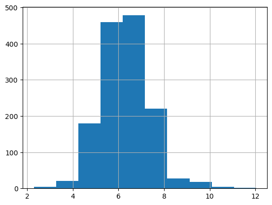

predictor_reg = TabularPredictor(label='TargetSales_log').fit(train_df_nonzero[selected_features+['TargetSales_log']],
                                                      presets=preset,
                                                      excluded_model_types=['NN_TORCH','FASTAI','KNN'],
                                                      )

No path specified. Models will be saved in: "AutogluonModels/ag-20241214_161346"
Verbosity: 2 (Standard Logging)
=================== System Info ===================
AutoGluon Version:  1.1.1
Python Version:     3.9.12
Operating System:   Linux
Platform Machine:   x86_64
Platform Version:   #1 SMP Wed Oct 23 01:22:11 UTC 2024
CPU Count:          64
Memory Avail:       466.78 GB / 480.23 GB (97.2%)
Disk Space Avail:   1450.75 GB / 1968.52 GB (73.7%)
===================================================
Presets specified: ['good_quality']
Setting dynamic_stacking from 'auto' to True. Reason: Enable dynamic_stacking when use_bag_holdout is disabled. (use_bag_holdout=False)
Stack configuration (auto_stack=True): num_stack_levels=1, num_bag_folds=8, num_bag_sets=1
Note: `save_bag_folds=False`! This will greatly reduce peak disk usage during fit (by ~8x), but runs the risk of an out-of-memory error during model refit if memory is small relative to the data size.
    You can avoid this risk by setting `save_bag_folds=True`.
DyStack is enabled (dynamic_stacking=True). AutoGluon will try to determine whether the input data is affected by stacked overfitting and enable or disable stacking as a consequence.
    This is used to identify the optimal `num_stack_levels` value. Copies of AutoGluon will be fit on subsets of the data. Then holdout validation data is used to detect stacked overfitting.
    Running DyStack for up to 900s of the 3600s of remaining time (25%).
/home/charipol/miniconda3/lib/python3.9/site-packages/autogluon/tabular/predictor/predictor.py:1242: UserWarning: Failed to use ray for memory safe fits. Falling back to normal fit. Error: ValueError('ray==2.40.0 detected. 2.10.0 <= ray < 2.11.0 is required. You can use pip to install certain version of ray `pip install ray==2.10.0` ')
  stacked_overfitting = self._sub_fit_memory_save_wrapper(
        Context path: "AutogluonModels/ag-20241214_161346/ds_sub_fit/sub_fit_ho"
Running DyStack sub-fit ...
Beginning AutoGluon training ... Time limit = 900s
AutoGluon will save models to "AutogluonModels/ag-20241214_161346/ds_sub_fit/sub_fit_ho"
Train Data Rows:    1256
Train Data Columns: 17
Label Column:       TargetSales_log
Problem Type:       regression
Preprocessing data ...
Using Feature Generators to preprocess the data ...
Fitting AutoMLPipelineFeatureGenerator...
    Available Memory:                    477983.00 MB
    Train Data (Original)  Memory Usage: 0.16 MB (0.0% of available memory)
    Inferring data type of each feature based on column values. Set feature_metadata_in to manually specify special dtypes of the features.
    Stage 1 Generators:
        Fitting AsTypeFeatureGenerator...
    Stage 2 Generators:
        Fitting FillNaFeatureGenerator...
    Stage 3 Generators:
        Fitting IdentityFeatureGenerator...
    Stage 4 Generators:
        Fitting DropUniqueFeatureGenerator...
    Stage 5 Generators:
        Fitting DropDuplicatesFeatureGenerator...
    Types of features in original data (raw dtype, special dtypes):
        ('float', []) : 12 | ['total_sales', 'avg_purchase_frequency', 'avg_purchase_value', 'per_fashion_accessories', 'per_home_decor', ...]
        ('int', [])   :  5 | ['recency', 'purchase_day', 'nb_product', 'nb_category', 'customer_lifetime']
    Types of features in processed data (raw dtype, special dtypes):
        ('float', []) : 12 | ['total_sales', 'avg_purchase_frequency', 'avg_purchase_value', 'per_fashion_accessories', 'per_home_decor', ...]
        ('int', [])   :  5 | ['recency', 'purchase_day', 'nb_product', 'nb_category', 'customer_lifetime']
    0.0s = Fit runtime
    17 features in original data used to generate 17 features in processed data.
    Train Data (Processed) Memory Usage: 0.16 MB (0.0% of available memory)
Data preprocessing and feature engineering runtime = 0.05s ...
AutoGluon will gauge predictive performance using evaluation metric: 'root_mean_squared_error'
    This metric's sign has been flipped to adhere to being higher_is_better. The metric score can be multiplied by -1 to get the metric value.
    To change this, specify the eval_metric parameter of Predictor()
User-specified model hyperparameters to be fit:
{
    'NN_TORCH': {},
    'GBM': [{'extra_trees': True, 'ag_args': {'name_suffix': 'XT'}}, {}, 'GBMLarge'],
    'CAT': {},
    'XGB': {},
    'FASTAI': {},
    'RF': [{'criterion': 'gini', 'max_depth': 15, 'ag_args': {'name_suffix': 'Gini', 'problem_types': ['binary', 'multiclass']}}, {'criterion': 'entropy', 'max_depth': 15, 'ag_args': {'name_suffix': 'Entr', 'problem_types': ['binary', 'multiclass']}}, {'criterion': 'squared_error', 'max_depth': 15, 'ag_args': {'name_suffix': 'MSE', 'problem_types': ['regression', 'quantile']}}],
    'XT': [{'criterion': 'gini', 'max_depth': 15, 'ag_args': {'name_suffix': 'Gini', 'problem_types': ['binary', 'multiclass']}}, {'criterion': 'entropy', 'max_depth': 15, 'ag_args': {'name_suffix': 'Entr', 'problem_types': ['binary', 'multiclass']}}, {'criterion': 'squared_error', 'max_depth': 15, 'ag_args': {'name_suffix': 'MSE', 'problem_types': ['regression', 'quantile']}}],
}
AutoGluon will fit 2 stack levels (L1 to L2) ...
Excluded models: ['NN_TORCH', 'FASTAI'] (Specified by `excluded_model_types`)
Fitting 7 L1 models ...
Fitting model: LightGBMXT_BAG_L1 ... Training model for up to 599.81s of the 899.94s of remaining time.
    Fitting 8 child models (S1F1 - S1F8) | Fitting with SequentialLocalFoldFittingStrategy
    -0.7829  = Validation score   (-root_mean_squared_error)
    5.83s    = Training   runtime
    0.01s    = Validation runtime
Fitting model: LightGBM_BAG_L1 ... Training model for up to 593.9s of the 894.03s of remaining time.
    Fitting 8 child models (S1F1 - S1F8) | Fitting with SequentialLocalFoldFittingStrategy
    -0.7864  = Validation score   (-root_mean_squared_error)
    5.68s    = Training   runtime
    0.01s    = Validation runtime
Fitting model: RandomForestMSE_BAG_L1 ... Training model for up to 588.14s of the 888.27s of remaining time.
    -0.8046  = Validation score   (-root_mean_squared_error)
    0.7s     = Training   runtime
    0.15s    = Validation runtime
Fitting model: CatBoost_BAG_L1 ... Training model for up to 587.17s of the 887.3s of remaining time.
    Fitting 8 child models (S1F1 - S1F8) | Fitting with SequentialLocalFoldFittingStrategy
    -0.7747  = Validation score   (-root_mean_squared_error)
    7.49s    = Training   runtime
    0.02s    = Validation runtime
Fitting model: ExtraTreesMSE_BAG_L1 ... Training model for up to 579.61s of the 879.74s of remaining time.
    -0.7815  = Validation score   (-root_mean_squared_error)
    0.62s    = Training   runtime
    0.15s    = Validation runtime
Fitting model: XGBoost_BAG_L1 ... Training model for up to 578.75s of the 878.88s of remaining time.
    Fitting 8 child models (S1F1 - S1F8) | Fitting with SequentialLocalFoldFittingStrategy
    -0.7865  = Validation score   (-root_mean_squared_error)
    5.41s    = Training   runtime
    0.03s    = Validation runtime
Fitting model: LightGBMLarge_BAG_L1 ... Training model for up to 573.25s of the 873.38s of remaining time.
    Fitting 8 child models (S1F1 - S1F8) | Fitting with SequentialLocalFoldFittingStrategy

[1000]  valid_set's rmse: 0.732165
[2000]  valid_set's rmse: 0.730646
[3000]  valid_set's rmse: 0.730279
[4000]  valid_set's rmse: 0.730248
[5000]  valid_set's rmse: 0.730238
[6000]  valid_set's rmse: 0.730238
[7000]  valid_set's rmse: 0.730238

    -0.8114  = Validation score   (-root_mean_squared_error)
    42.21s   = Training   runtime
    0.03s    = Validation runtime
Fitting model: WeightedEnsemble_L2 ... Training model for up to 360.0s of the 831.05s of remaining time.
    Ensemble Weights: {'CatBoost_BAG_L1': 0.455, 'ExtraTreesMSE_BAG_L1': 0.227, 'XGBoost_BAG_L1': 0.182, 'LightGBM_BAG_L1': 0.136}
    -0.7698  = Validation score   (-root_mean_squared_error)
    0.02s    = Training   runtime
    0.0s     = Validation runtime
Excluded models: ['NN_TORCH', 'FASTAI'] (Specified by `excluded_model_types`)
Fitting 7 L2 models ...
Fitting model: LightGBMXT_BAG_L2 ... Training model for up to 830.98s of the 830.98s of remaining time.
    Fitting 8 child models (S1F1 - S1F8) | Fitting with SequentialLocalFoldFittingStrategy
    -0.7955  = Validation score   (-root_mean_squared_error)
    5.59s    = Training   runtime
    0.01s    = Validation runtime
Fitting model: LightGBM_BAG_L2 ... Training model for up to 825.34s of the 825.33s of remaining time.
    Fitting 8 child models (S1F1 - S1F8) | Fitting with SequentialLocalFoldFittingStrategy

[1000]  valid_set's rmse: 0.776795

    -0.7972  = Validation score   (-root_mean_squared_error)
    7.51s    = Training   runtime
    0.01s    = Validation runtime
Fitting model: RandomForestMSE_BAG_L2 ... Training model for up to 817.73s of the 817.72s of remaining time.
    -0.8017  = Validation score   (-root_mean_squared_error)
    0.67s    = Training   runtime
    0.15s    = Validation runtime
Fitting model: CatBoost_BAG_L2 ... Training model for up to 816.81s of the 816.8s of remaining time.
    Fitting 8 child models (S1F1 - S1F8) | Fitting with SequentialLocalFoldFittingStrategy
    -0.7824  = Validation score   (-root_mean_squared_error)
    5.55s    = Training   runtime
    0.02s    = Validation runtime
Fitting model: ExtraTreesMSE_BAG_L2 ... Training model for up to 811.18s of the 811.18s of remaining time.
    -0.7873  = Validation score   (-root_mean_squared_error)
    0.61s    = Training   runtime
    0.15s    = Validation runtime
Fitting model: XGBoost_BAG_L2 ... Training model for up to 810.31s of the 810.3s of remaining time.
    Fitting 8 child models (S1F1 - S1F8) | Fitting with SequentialLocalFoldFittingStrategy
    -0.8012  = Validation score   (-root_mean_squared_error)
    6.75s    = Training   runtime
    0.03s    = Validation runtime
Fitting model: LightGBMLarge_BAG_L2 ... Training model for up to 803.46s of the 803.45s of remaining time.
    Fitting 8 child models (S1F1 - S1F8) | Fitting with SequentialLocalFoldFittingStrategy
    -0.8115  = Validation score   (-root_mean_squared_error)
    15.94s   = Training   runtime
    0.01s    = Validation runtime
Fitting model: WeightedEnsemble_L3 ... Training model for up to 360.0s of the 787.41s of remaining time.
    Ensemble Weights: {'CatBoost_BAG_L1': 0.412, 'ExtraTreesMSE_BAG_L1': 0.176, 'LightGBM_BAG_L1': 0.118, 'XGBoost_BAG_L1': 0.118, 'XGBoost_BAG_L2': 0.118, 'LightGBM_BAG_L2': 0.059}
    -0.7689  = Validation score   (-root_mean_squared_error)
    0.03s    = Training   runtime
    0.0s     = Validation runtime
AutoGluon training complete, total runtime = 112.67s ... Best model: WeightedEnsemble_L3 | Estimated inference throughput: 945.3 rows/s (157 batch size)
Automatically performing refit_full as a post-fit operation (due to `.fit(..., refit_full=True)`
Refitting models via `predictor.refit_full` using all of the data (combined train and validation)...
    Models trained in this way will have the suffix "_FULL" and have NaN validation score.
    This process is not bound by time_limit, but should take less time than the original `predictor.fit` call.
    To learn more, refer to the `.refit_full` method docstring which explains how "_FULL" models differ from normal models.
Fitting 1 L1 models ...
Fitting model: LightGBMXT_BAG_L1_FULL ...
    0.43s    = Training   runtime
Fitting 1 L1 models ...
Fitting model: LightGBM_BAG_L1_FULL ...
    0.4s     = Training   runtime
Fitting model: RandomForestMSE_BAG_L1_FULL | Skipping fit via cloning parent ...
    0.7s     = Training   runtime
    0.15s    = Validation runtime
Fitting 1 L1 models ...
Fitting model: CatBoost_BAG_L1_FULL ...
    0.38s    = Training   runtime
Fitting model: ExtraTreesMSE_BAG_L1_FULL | Skipping fit via cloning parent ...
    0.62s    = Training   runtime
    0.15s    = Validation runtime
Fitting 1 L1 models ...
Fitting model: XGBoost_BAG_L1_FULL ...
    0.13s    = Training   runtime
Fitting 1 L1 models ...
Fitting model: LightGBMLarge_BAG_L1_FULL ...
    3.38s    = Training   runtime
Fitting model: WeightedEnsemble_L2_FULL | Skipping fit via cloning parent ...
    Ensemble Weights: {'CatBoost_BAG_L1': 0.455, 'ExtraTreesMSE_BAG_L1': 0.227, 'XGBoost_BAG_L1': 0.182, 'LightGBM_BAG_L1': 0.136}
    0.02s    = Training   runtime
Fitting 1 L2 models ...
Fitting model: LightGBMXT_BAG_L2_FULL ...
    0.4s     = Training   runtime
Fitting 1 L2 models ...
Fitting model: LightGBM_BAG_L2_FULL ...
    0.61s    = Training   runtime
Fitting model: RandomForestMSE_BAG_L2_FULL | Skipping fit via cloning parent ...
    0.67s    = Training   runtime
    0.15s    = Validation runtime
Fitting 1 L2 models ...
Fitting model: CatBoost_BAG_L2_FULL ...
    0.2s     = Training   runtime
Fitting model: ExtraTreesMSE_BAG_L2_FULL | Skipping fit via cloning parent ...
    0.61s    = Training   runtime
    0.15s    = Validation runtime
Fitting 1 L2 models ...
Fitting model: XGBoost_BAG_L2_FULL ...
    0.3s     = Training   runtime
Fitting 1 L2 models ...
Fitting model: LightGBMLarge_BAG_L2_FULL ...
    0.84s    = Training   runtime
Fitting model: WeightedEnsemble_L3_FULL | Skipping fit via cloning parent ...
    Ensemble Weights: {'CatBoost_BAG_L1': 0.412, 'ExtraTreesMSE_BAG_L1': 0.176, 'LightGBM_BAG_L1': 0.118, 'XGBoost_BAG_L1': 0.118, 'XGBoost_BAG_L2': 0.118, 'LightGBM_BAG_L2': 0.059}
    0.03s    = Training   runtime
Updated best model to "WeightedEnsemble_L3_FULL" (Previously "WeightedEnsemble_L3"). AutoGluon will default to using "WeightedEnsemble_L3_FULL" for predict() and predict_proba().
Refit complete, total runtime = 7.83s ... Best model: "WeightedEnsemble_L3_FULL"
TabularPredictor saved. To load, use: predictor = TabularPredictor.load("AutogluonModels/ag-20241214_161346/ds_sub_fit/sub_fit_ho")
Deleting DyStack predictor artifacts (clean_up_fits=True) ...
Leaderboard on holdout data (DyStack):
                          model  score_holdout  score_val              eval_metric  pred_time_test  pred_time_val  fit_time  pred_time_test_marginal  pred_time_val_marginal  fit_time_marginal  stack_level  can_infer  fit_order
0     ExtraTreesMSE_BAG_L1_FULL      -0.839346  -0.781522  root_mean_squared_error        0.130818       0.146218  0.616536                 0.130818                0.146218           0.616536            1       True          5
1     ExtraTreesMSE_BAG_L2_FULL      -0.853589  -0.787303  root_mean_squared_error        0.446297            NaN  6.640192                 0.132555                0.153409           0.613806            2       True         13
2      WeightedEnsemble_L3_FULL      -0.857556  -0.768871  root_mean_squared_error        0.340568            NaN  6.967287                 0.005255                     NaN           0.026960            3       True         16
3   RandomForestMSE_BAG_L1_FULL      -0.861175  -0.804629  root_mean_squared_error        0.122124       0.147519  0.702981                 0.122124                0.147519           0.702981            1       True          3
4      WeightedEnsemble_L2_FULL      -0.862117  -0.769820  root_mean_squared_error        0.157042            NaN  1.533079                 0.004246                     NaN           0.017303            2       True          8
5        LightGBMXT_BAG_L1_FULL      -0.864283  -0.782882  root_mean_squared_error        0.002461            NaN  0.427038                 0.002461                     NaN           0.427038            1       True          1
6          CatBoost_BAG_L2_FULL      -0.866735  -0.782409  root_mean_squared_error        0.322393            NaN  6.225857                 0.008651                     NaN           0.199471            2       True         12
7   RandomForestMSE_BAG_L2_FULL      -0.867588  -0.801697  root_mean_squared_error        0.442486            NaN  6.695999                 0.128743                0.152188           0.669613            2       True         11
8        LightGBMXT_BAG_L2_FULL      -0.867632  -0.795484  root_mean_squared_error        0.317761            NaN  6.431228                 0.004019                     NaN           0.404842            2       True          9
9           XGBoost_BAG_L2_FULL      -0.867990  -0.801243  root_mean_squared_error        0.327944            NaN  6.329812                 0.014201                     NaN           0.303426            2       True         14
10         LightGBM_BAG_L2_FULL      -0.869884  -0.797155  root_mean_squared_error        0.321112            NaN  6.636901                 0.007370                     NaN           0.610516            2       True         10
11         LightGBM_BAG_L1_FULL      -0.872511  -0.786431  root_mean_squared_error        0.001978            NaN  0.396514                 0.001978                     NaN           0.396514            1       True          2
12         CatBoost_BAG_L1_FULL      -0.876613  -0.774745  root_mean_squared_error        0.007943            NaN  0.375822                 0.007943                     NaN           0.375822            1       True          4
13          XGBoost_BAG_L1_FULL      -0.908105  -0.786510  root_mean_squared_error        0.012056            NaN  0.126903                 0.012056                     NaN           0.126903            1       True          6
14    LightGBMLarge_BAG_L2_FULL      -0.929002  -0.811482  root_mean_squared_error        0.322513            NaN  6.862701                 0.008771                     NaN           0.836315            2       True         15
15    LightGBMLarge_BAG_L1_FULL      -0.943116  -0.811385  root_mean_squared_error        0.036361            NaN  3.380592                 0.036361                     NaN           3.380592            1       True          7
    1    = Optimal   num_stack_levels (Stacked Overfitting Occurred: False)
    121s     = DyStack   runtime |  3479s    = Remaining runtime
Starting main fit with num_stack_levels=1.
    For future fit calls on this dataset, you can skip DyStack to save time: `predictor.fit(..., dynamic_stacking=False, num_stack_levels=1)`
Beginning AutoGluon training ... Time limit = 3479s
AutoGluon will save models to "AutogluonModels/ag-20241214_161346"
Train Data Rows:    1414
Train Data Columns: 17
Label Column:       TargetSales_log
Problem Type:       regression
Preprocessing data ...
Using Feature Generators to preprocess the data ...
Fitting AutoMLPipelineFeatureGenerator...
    Available Memory:                    478011.59 MB
    Train Data (Original)  Memory Usage: 0.18 MB (0.0% of available memory)
    Inferring data type of each feature based on column values. Set feature_metadata_in to manually specify special dtypes of the features.
    Stage 1 Generators:
        Fitting AsTypeFeatureGenerator...
    Stage 2 Generators:
        Fitting FillNaFeatureGenerator...
    Stage 3 Generators:
        Fitting IdentityFeatureGenerator...
    Stage 4 Generators:
        Fitting DropUniqueFeatureGenerator...
    Stage 5 Generators:
        Fitting DropDuplicatesFeatureGenerator...
    Types of features in original data (raw dtype, special dtypes):
        ('float', []) : 12 | ['total_sales', 'avg_purchase_frequency', 'avg_purchase_value', 'per_fashion_accessories', 'per_home_decor', ...]
        ('int', [])   :  5 | ['recency', 'purchase_day', 'nb_product', 'nb_category', 'customer_lifetime']
    Types of features in processed data (raw dtype, special dtypes):
        ('float', []) : 12 | ['total_sales', 'avg_purchase_frequency', 'avg_purchase_value', 'per_fashion_accessories', 'per_home_decor', ...]
        ('int', [])   :  5 | ['recency', 'purchase_day', 'nb_product', 'nb_category', 'customer_lifetime']
    0.0s = Fit runtime
    17 features in original data used to generate 17 features in processed data.
    Train Data (Processed) Memory Usage: 0.18 MB (0.0% of available memory)
Data preprocessing and feature engineering runtime = 0.06s ...
AutoGluon will gauge predictive performance using evaluation metric: 'root_mean_squared_error'
    This metric's sign has been flipped to adhere to being higher_is_better. The metric score can be multiplied by -1 to get the metric value.
    To change this, specify the eval_metric parameter of Predictor()
User-specified model hyperparameters to be fit:
{
    'NN_TORCH': {},
    'GBM': [{'extra_trees': True, 'ag_args': {'name_suffix': 'XT'}}, {}, 'GBMLarge'],
    'CAT': {},
    'XGB': {},
    'FASTAI': {},
    'RF': [{'criterion': 'gini', 'max_depth': 15, 'ag_args': {'name_suffix': 'Gini', 'problem_types': ['binary', 'multiclass']}}, {'criterion': 'entropy', 'max_depth': 15, 'ag_args': {'name_suffix': 'Entr', 'problem_types': ['binary', 'multiclass']}}, {'criterion': 'squared_error', 'max_depth': 15, 'ag_args': {'name_suffix': 'MSE', 'problem_types': ['regression', 'quantile']}}],
    'XT': [{'criterion': 'gini', 'max_depth': 15, 'ag_args': {'name_suffix': 'Gini', 'problem_types': ['binary', 'multiclass']}}, {'criterion': 'entropy', 'max_depth': 15, 'ag_args': {'name_suffix': 'Entr', 'problem_types': ['binary', 'multiclass']}}, {'criterion': 'squared_error', 'max_depth': 15, 'ag_args': {'name_suffix': 'MSE', 'problem_types': ['regression', 'quantile']}}],
}
AutoGluon will fit 2 stack levels (L1 to L2) ...
Excluded models: ['NN_TORCH', 'FASTAI'] (Specified by `excluded_model_types`)
Fitting 7 L1 models ...
Fitting model: LightGBMXT_BAG_L1 ... Training model for up to 2318.53s of the 3478.66s of remaining time.
    Fitting 8 child models (S1F1 - S1F8) | Fitting with SequentialLocalFoldFittingStrategy
    -0.7909  = Validation score   (-root_mean_squared_error)
    5.92s    = Training   runtime
    0.01s    = Validation runtime
Fitting model: LightGBM_BAG_L1 ... Training model for up to 2312.52s of the 3472.65s of remaining time.
    Fitting 8 child models (S1F1 - S1F8) | Fitting with SequentialLocalFoldFittingStrategy
    -0.7919  = Validation score   (-root_mean_squared_error)
    5.67s    = Training   runtime
    0.01s    = Validation runtime
Fitting model: RandomForestMSE_BAG_L1 ... Training model for up to 2306.77s of the 3466.9s of remaining time.
    -0.8074  = Validation score   (-root_mean_squared_error)
    0.67s    = Training   runtime
    0.15s    = Validation runtime
Fitting model: CatBoost_BAG_L1 ... Training model for up to 2305.84s of the 3465.97s of remaining time.
    Fitting 8 child models (S1F1 - S1F8) | Fitting with SequentialLocalFoldFittingStrategy
    -0.783   = Validation score   (-root_mean_squared_error)
    6.6s     = Training   runtime
    0.02s    = Validation runtime
Fitting model: ExtraTreesMSE_BAG_L1 ... Training model for up to 2299.16s of the 3459.29s of remaining time.
    -0.7902  = Validation score   (-root_mean_squared_error)
    0.6s     = Training   runtime
    0.15s    = Validation runtime
Fitting model: XGBoost_BAG_L1 ... Training model for up to 2298.3s of the 3458.44s of remaining time.
    Fitting 8 child models (S1F1 - S1F8) | Fitting with SequentialLocalFoldFittingStrategy
    -0.8026  = Validation score   (-root_mean_squared_error)
    5.14s    = Training   runtime
    0.02s    = Validation runtime
Fitting model: LightGBMLarge_BAG_L1 ... Training model for up to 2293.07s of the 3453.2s of remaining time.
    Fitting 8 child models (S1F1 - S1F8) | Fitting with SequentialLocalFoldFittingStrategy
    -0.8166  = Validation score   (-root_mean_squared_error)
    14.87s   = Training   runtime
    0.01s    = Validation runtime
Fitting model: WeightedEnsemble_L2 ... Training model for up to 360.0s of the 3438.24s of remaining time.
    Ensemble Weights: {'CatBoost_BAG_L1': 0.5, 'ExtraTreesMSE_BAG_L1': 0.25, 'LightGBM_BAG_L1': 0.188, 'LightGBMXT_BAG_L1': 0.062}
    -0.78    = Validation score   (-root_mean_squared_error)
    0.02s    = Training   runtime
    0.0s     = Validation runtime
Excluded models: ['NN_TORCH', 'FASTAI'] (Specified by `excluded_model_types`)
Fitting 7 L2 models ...
Fitting model: LightGBMXT_BAG_L2 ... Training model for up to 3438.17s of the 3438.16s of remaining time.
    Fitting 8 child models (S1F1 - S1F8) | Fitting with SequentialLocalFoldFittingStrategy

[1000]  valid_set's rmse: 0.741321
[2000]  valid_set's rmse: 0.735104
[1000]  valid_set's rmse: 0.756407
[1000]  valid_set's rmse: 0.712855

    -0.7869  = Validation score   (-root_mean_squared_error)
    9.95s    = Training   runtime
    0.01s    = Validation runtime
Fitting model: LightGBM_BAG_L2 ... Training model for up to 3428.15s of the 3428.14s of remaining time.
    Fitting 8 child models (S1F1 - S1F8) | Fitting with SequentialLocalFoldFittingStrategy
    -0.7932  = Validation score   (-root_mean_squared_error)
    6.95s    = Training   runtime
    0.01s    = Validation runtime
Fitting model: RandomForestMSE_BAG_L2 ... Training model for up to 3421.11s of the 3421.1s of remaining time.
    -0.8097  = Validation score   (-root_mean_squared_error)
    0.7s     = Training   runtime
    0.15s    = Validation runtime
Fitting model: CatBoost_BAG_L2 ... Training model for up to 3420.15s of the 3420.15s of remaining time.
    Fitting 8 child models (S1F1 - S1F8) | Fitting with SequentialLocalFoldFittingStrategy
    -0.7847  = Validation score   (-root_mean_squared_error)
    9.03s    = Training   runtime
    0.02s    = Validation runtime
Fitting model: ExtraTreesMSE_BAG_L2 ... Training model for up to 3411.04s of the 3411.04s of remaining time.
    -0.795   = Validation score   (-root_mean_squared_error)
    0.6s     = Training   runtime
    0.15s    = Validation runtime
Fitting model: XGBoost_BAG_L2 ... Training model for up to 3410.19s of the 3410.18s of remaining time.
    Fitting 8 child models (S1F1 - S1F8) | Fitting with SequentialLocalFoldFittingStrategy
    -0.8102  = Validation score   (-root_mean_squared_error)
    6.21s    = Training   runtime
    0.04s    = Validation runtime
Fitting model: LightGBMLarge_BAG_L2 ... Training model for up to 3403.88s of the 3403.87s of remaining time.
    Fitting 8 child models (S1F1 - S1F8) | Fitting with SequentialLocalFoldFittingStrategy

[1000]  valid_set's rmse: 0.75982
[2000]  valid_set's rmse: 0.759573
[1000]  valid_set's rmse: 0.838684
[2000]  valid_set's rmse: 0.838386

    -0.8107  = Validation score   (-root_mean_squared_error)
    31.41s   = Training   runtime
    0.02s    = Validation runtime
Fitting model: WeightedEnsemble_L3 ... Training model for up to 360.0s of the 3372.32s of remaining time.
    Ensemble Weights: {'CatBoost_BAG_L1': 0.333, 'LightGBMXT_BAG_L2': 0.25, 'LightGBM_BAG_L2': 0.167, 'LightGBM_BAG_L1': 0.083, 'ExtraTreesMSE_BAG_L1': 0.083, 'LightGBMLarge_BAG_L2': 0.083}
    -0.7746  = Validation score   (-root_mean_squared_error)
    0.04s    = Training   runtime
    0.0s     = Validation runtime
AutoGluon training complete, total runtime = 106.52s ... Best model: WeightedEnsemble_L3 | Estimated inference throughput: 1175.2 rows/s (177 batch size)
Automatically performing refit_full as a post-fit operation (due to `.fit(..., refit_full=True)`
Refitting models via `predictor.refit_full` using all of the data (combined train and validation)...
    Models trained in this way will have the suffix "_FULL" and have NaN validation score.
    This process is not bound by time_limit, but should take less time than the original `predictor.fit` call.
    To learn more, refer to the `.refit_full` method docstring which explains how "_FULL" models differ from normal models.
Fitting 1 L1 models ...
Fitting model: LightGBMXT_BAG_L1_FULL ...
    0.43s    = Training   runtime
Fitting 1 L1 models ...
Fitting model: LightGBM_BAG_L1_FULL ...
    0.4s     = Training   runtime
Fitting model: RandomForestMSE_BAG_L1_FULL | Skipping fit via cloning parent ...
    0.67s    = Training   runtime
    0.15s    = Validation runtime
Fitting 1 L1 models ...
Fitting model: CatBoost_BAG_L1_FULL ...
    0.29s    = Training   runtime
Fitting model: ExtraTreesMSE_BAG_L1_FULL | Skipping fit via cloning parent ...
    0.6s     = Training   runtime
    0.15s    = Validation runtime
Fitting 1 L1 models ...
Fitting model: XGBoost_BAG_L1_FULL ...
    0.09s    = Training   runtime
Fitting 1 L1 models ...
Fitting model: LightGBMLarge_BAG_L1_FULL ...
    0.73s    = Training   runtime
Fitting model: WeightedEnsemble_L2_FULL | Skipping fit via cloning parent ...
    Ensemble Weights: {'CatBoost_BAG_L1': 0.5, 'ExtraTreesMSE_BAG_L1': 0.25, 'LightGBM_BAG_L1': 0.188, 'LightGBMXT_BAG_L1': 0.062}
    0.02s    = Training   runtime
Fitting 1 L2 models ...
Fitting model: LightGBMXT_BAG_L2_FULL ...
    0.83s    = Training   runtime
Fitting 1 L2 models ...
Fitting model: LightGBM_BAG_L2_FULL ...
    0.54s    = Training   runtime
Fitting model: RandomForestMSE_BAG_L2_FULL | Skipping fit via cloning parent ...
    0.7s     = Training   runtime
    0.15s    = Validation runtime
Fitting 1 L2 models ...
Fitting model: CatBoost_BAG_L2_FULL ...
    0.39s    = Training   runtime
Fitting model: ExtraTreesMSE_BAG_L2_FULL | Skipping fit via cloning parent ...
    0.6s     = Training   runtime
    0.15s    = Validation runtime
Fitting 1 L2 models ...
Fitting model: XGBoost_BAG_L2_FULL ...
    0.18s    = Training   runtime
Fitting 1 L2 models ...
Fitting model: LightGBMLarge_BAG_L2_FULL ...
    2.46s    = Training   runtime
Fitting model: WeightedEnsemble_L3_FULL | Skipping fit via cloning parent ...
    Ensemble Weights: {'CatBoost_BAG_L1': 0.333, 'LightGBMXT_BAG_L2': 0.25, 'LightGBM_BAG_L2': 0.167, 'LightGBM_BAG_L1': 0.083, 'ExtraTreesMSE_BAG_L1': 0.083, 'LightGBMLarge_BAG_L2': 0.083}
    0.04s    = Training   runtime
Updated best model to "WeightedEnsemble_L3_FULL" (Previously "WeightedEnsemble_L3"). AutoGluon will default to using "WeightedEnsemble_L3_FULL" for predict() and predict_proba().
Refit complete, total runtime = 7.11s ... Best model: "WeightedEnsemble_L3_FULL"
TabularPredictor saved. To load, use: predictor = TabularPredictor.load("AutogluonModels/ag-20241214_161346")

test_df_nonzero['pred_log'] = predictor_reg.predict(test_df_nonzero[selected_features])
test_df_nonzero['pred_log_exp'] = test_df_nonzero['pred_log'].map(np.exp)

test_df['pred_log'] = predictor_reg.predict(test_df[selected_features])
test_df['pred_log_exp'] = test_df['pred_log'].map(np.exp)

calculate_regression_metrics(test_df_nonzero['TargetSales'], test_df_nonzero['pred_log_exp'])

{'root_mean_squared_error': 4330.443144695726,
 'mean_squared_error': 18752737.82944221,
 'mean_absolute_error': 880.0418223064565,
 'r2': 0.3647576298877435,
 'pearsonr': 0.6756393928483335,
 'spearmanr': 0.5762190201444638,
 'median_absolute_error': 243.0658528752748,
 'earths_mover_distance': 546.7166312173882}

test_df['pred_hurdle'] = test_df.pred_binary * test_df.pred_log_exp

metric_hurdle = calculate_regression_metrics(test_df['TargetSales'], test_df['pred_hurdle'])
metric_hurdle['model'] = 'hurdle'
metric_hurdle

{'root_mean_squared_error': 3171.760744960863,
 'mean_squared_error': 10060066.22327469,
 'mean_absolute_error': 584.9162934881963,
 'r2': 0.3779813431428882,
 'pearsonr': 0.6769697889999318,
 'spearmanr': 0.5107083593715698,
 'median_absolute_error': 199.1780137692856,
 'earths_mover_distance': 286.381442541919,
 'model': 'hurdle'}

Duan’s Method

When predicting a log-transformed outcome, we typically want to re-transform the predictions to non-log numbers by applying the exponential function. However, this ignores a small bias due to the error term in the process.

\[ln(y) = f(X) + \epsilon\]

where * \(y\) is actual outcome. * \(X\) is the features. * \(f(.)\) is a trained model. * \(\epsilon\) is the error term.

when re-transforming \[ \begin{align} y &= exp(ln(y)) \\ &= exp(f(X) + \epsilon ) \\ &= exp(f(X)) \cdot exp(\epsilon) \\ E[y] &= E[exp(f(X))] \cdot E[exp(\epsilon)] \end{align} \]

Duan estimates the E[\(exp(\epsilon)\)] as \[ \begin{align} \hat \lambda &= E[exp(ln(y) - ln(\hat y))] \end{align} \]

where * \(\hat \lambda\) is the Duan’s smearing estimator of the bias from re-transformation \(E[exp(\epsilon)]\) * \(\hat y\) is the prediction aka \(f(X)\)

train_df_nonzero['pred_log'] = predictor_reg.predict(train_df_nonzero[selected_features])
train_df_nonzero['pred_log_exp'] = train_df_nonzero['pred_log'].map(np.exp)

smearing_estimator = np.mean(np.exp(train_df_nonzero['TargetSales_log'] - train_df_nonzero['pred_log']))
smearing_estimator

1.2280991653046711

np.exp(train_df_nonzero['TargetSales_log'] - train_df_nonzero['pred_log']).hist()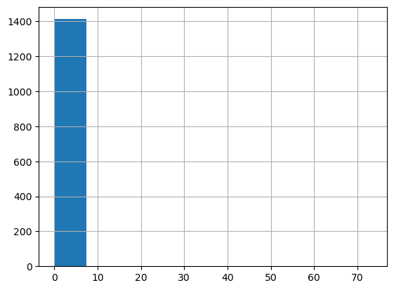

test_df['pred_log_exp_corrected'] = test_df['pred_log_exp'] * smearing_estimator
test_df['pred_hurdle_corrected'] = test_df.pred_binary * test_df.pred_log_exp_corrected

metric_hurdle_corrected = calculate_regression_metrics(test_df['TargetSales'], test_df['pred_hurdle_corrected'])
metric_hurdle_corrected['model'] = 'hurdle_corrected'
metric_hurdle_corrected

{'root_mean_squared_error': 3055.3207868281233,
 'mean_squared_error': 9334985.110424023,
 'mean_absolute_error': 613.3946643257099,
 'r2': 0.42281345159207295,
 'pearsonr': 0.6769697889999318,
 'spearmanr': 0.5107083593715698,
 'median_absolute_error': 232.55557358084502,
 'earths_mover_distance': 241.61839859133218,
 'model': 'hurdle_corrected'}

Assumption on Independent and Identically Distributed Residuals

But not so fast, the formulation of Duan’s smearing estimator assumes that estimates of error terms (residuals) for log predictions be independent and identically distributed. Since we are dealing with individual customers, independence can be assumed. However, if we look at the plot of residuals vs predicted log values, we can see that they are not identically distributed.

#plot residual and predicted log value
train_df_nonzero['pred_log'] = predictor_reg.predict(train_df_nonzero[selected_features])
train_df_nonzero['residual_log'] = (train_df_nonzero['pred_log'] - train_df_nonzero['TargetSales_log'])

# Create the scatter plot
sns.scatterplot(x='pred_log', y='residual_log', data=train_df_nonzero)

# Add the Lowess smoothing line
sns.regplot(x='pred_log', y='residual_log', data=train_df_nonzero, scatter_kws={'alpha': 0.5}, line_kws={'color': 'red'})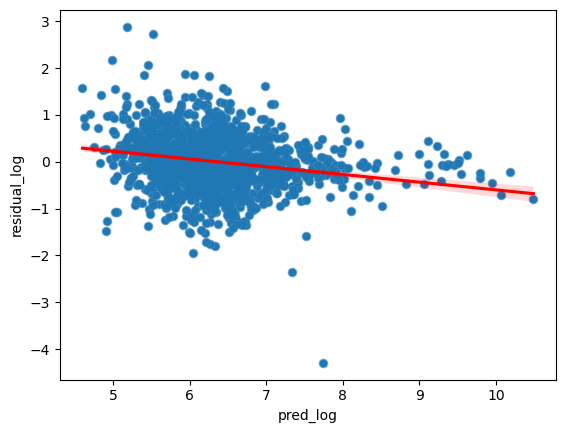

Although note that White test does not reject the null hypothesis of the residuals being homoscedastic in reference to the features. This counterintuitive result might stem from the fact that White test is assuming linear or quadratic relationships between outcome and features while the residuals are derived from a stacked ensemble of decision trees.

white_stat, white_p_value, _, _ = het_white(train_df_nonzero['residual_log'], 
                                            train_df_nonzero[selected_features])
print(f"White Test Statistic: {white_stat}")
print(f"P-value: {white_p_value}")

White Test Statistic: 129.31318320644837
P-value: 0.8761278601130765

Our choice is to either trust the White test and pretend assume everything is fine; or trust our eyes and replace the non-zero regression model with one that produces iid residuals such as generalized least squares (GLS) with heteroscedasticity-robust standard errors. In order to satisfy the assumptions of GLS, we perform winsorization, standardization and verify multicollinearity among the features.

train_df_nonzero_processed = train_df_nonzero.copy()

#winsorize at 99%
winsorizer = Winsorizer(cols=selected_features, percentile=99)
winsorizer.fit(train_df_nonzero_processed)
train_df_nonzero_processed = winsorizer.transform(train_df_nonzero_processed)

#standard scaling
scaler = StandardScaler()
scaler.fit(train_df_nonzero_processed[selected_features])
train_df_nonzero_processed[selected_features] = scaler.transform(train_df_nonzero_processed[selected_features])

#check vif
vif_data = calculate_vif(train_df_nonzero_processed, selected_features)

# Print the VIF for each feature
print(vif_data)

# Filter out features with high VIF (e.g., VIF > 10 suggests multicollinearity)
high_vif_features = vif_data[vif_data['VIF'] > 10]
print("High VIF features:", high_vif_features)

                           feature        VIF
0                            const   1.000000
1                          recency   3.976800
2                     purchase_day   6.193391
3                      total_sales   5.837235
4                       nb_product   2.386644
5                      nb_category   2.691338
6                customer_lifetime   2.271404
7           avg_purchase_frequency   5.291575
8               avg_purchase_value   2.449152
9          per_fashion_accessories   5.826894
10                  per_home_decor  15.806683
11          per_kitchen_and_dining  12.053308
12                      per_others   1.779531
13          per_outdoor_and_garden   2.729103
14  per_personal_care_and_wellness   2.908001
15        per_seasonal_and_holiday   4.234883
16        per_stationary_and_gifts   4.252687
17              per_toys_and_games   3.185269
High VIF features:                    feature        VIF
10          per_home_decor  15.806683
11  per_kitchen_and_dining  12.053308

# Calculate VIF after dropping highly correlated features
selected_features_no_corr = [i for i in selected_features if i!='per_kitchen_and_dining']
vif_data = calculate_vif(train_df_nonzero_processed.drop('per_kitchen_and_dining',axis=1), 
                         selected_features_no_corr)

# Print the VIF for each feature
print(vif_data)

# Filter out features with high VIF (e.g., VIF > 10 suggests multicollinearity)
high_vif_features = vif_data[vif_data['VIF'] > 10]
print("High VIF features:", high_vif_features)

                           feature       VIF
0                            const  1.000000
1                          recency  3.975755
2                     purchase_day  6.193274
3                      total_sales  5.835455
4                       nb_product  2.355212
5                      nb_category  2.238039
6                customer_lifetime  2.265888
7           avg_purchase_frequency  5.288665
8               avg_purchase_value  2.447088
9          per_fashion_accessories  1.271944
10                  per_home_decor  1.642046
11                      per_others  1.172240
12          per_outdoor_and_garden  1.122673
13  per_personal_care_and_wellness  1.141183
14        per_seasonal_and_holiday  1.180130
15        per_stationary_and_gifts  1.310125
16              per_toys_and_games  1.198112
High VIF features: Empty DataFrame
Columns: [feature, VIF]
Index: []

y = train_df_nonzero_processed['TargetSales_log']
X = train_df_nonzero_processed[selected_features_no_corr]
X = sm.add_constant(X)

gls_model = sm.GLS(y, X)
gls_results = gls_model.fit(cov_type='HC3')

# 4. Print the summary of the regression
print(gls_results.summary())

                            GLS Regression Results                            
==============================================================================
Dep. Variable:        TargetSales_log   R-squared:                       0.460
Model:                            GLS   Adj. R-squared:                  0.454
Method:                 Least Squares   F-statistic:                     75.24
Date:                Sat, 14 Dec 2024   Prob (F-statistic):          2.27e-175
Time:                        16:56:46   Log-Likelihood:                -1661.3
No. Observations:                1414   AIC:                             3357.
Df Residuals:                    1397   BIC:                             3446.
Df Model:                          16                                         
Covariance Type:                  HC3                                         
==================================================================================================
                                     coef    std err          z      P>|z|      [0.025      0.975]
--------------------------------------------------------------------------------------------------
const                              6.3127      0.021    299.031      0.000       6.271       6.354
recency                            0.0054      0.047      0.114      0.909      -0.087       0.098
purchase_day                       0.3697      0.046      7.977      0.000       0.279       0.460
total_sales                        0.1438      0.049      2.905      0.004       0.047       0.241
nb_product                        -0.0293      0.032     -0.929      0.353      -0.091       0.033
nb_category                        0.1163      0.034      3.448      0.001       0.050       0.182
customer_lifetime                 -0.0170      0.032     -0.524      0.600      -0.081       0.047
avg_purchase_frequency            -0.0103      0.052     -0.197      0.844      -0.113       0.092
avg_purchase_value                 0.3817      0.034     11.257      0.000       0.315       0.448
per_fashion_accessories           -0.0216      0.030     -0.724      0.469      -0.080       0.037
per_home_decor                    -0.0063      0.034     -0.188      0.851      -0.072       0.060
per_others                        -0.0165      0.023     -0.706      0.480      -0.062       0.029
per_outdoor_and_garden            -0.0397      0.022     -1.768      0.077      -0.084       0.004
per_personal_care_and_wellness    -0.0042      0.025     -0.167      0.867      -0.054       0.045
per_seasonal_and_holiday          -0.0796      0.025     -3.248      0.001      -0.128      -0.032
per_stationary_and_gifts           0.0166      0.024      0.698      0.485      -0.030       0.063
per_toys_and_games                -0.0230      0.026     -0.900      0.368      -0.073       0.027
==============================================================================
Omnibus:                      162.402   Durbin-Watson:                   2.022
Prob(Omnibus):                  0.000   Jarque-Bera (JB):             1272.986
Skew:                           0.198   Prob(JB):                    3.75e-277
Kurtosis:                       7.631   Cond. No.                         6.59
==============================================================================

Notes:
[1] Standard Errors are heteroscedasticity robust (HC3)

#plot residual and predicted log value
train_df_nonzero_processed['pred_log_gls'] = gls_results.predict(X).reset_index(drop=True)
train_df_nonzero_processed['residual_log_gls'] = (train_df_nonzero_processed['pred_log_gls'] - train_df_nonzero_processed['TargetSales_log'])
train_df_nonzero_processed.plot.scatter(x='pred_log_gls', y='residual_log_gls')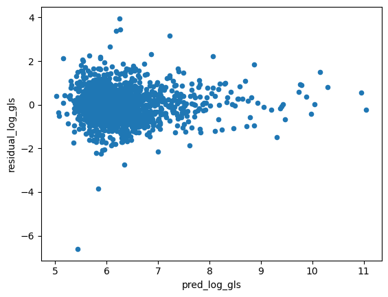

white_stat, white_p_value, _, _ = het_white(train_df_nonzero_processed['residual_log_gls'], 
                                            X)
print(f"White Test Statistic: {white_stat}")
print(f"P-value: {white_p_value}")

White Test Statistic: 135.0623196454856
P-value: 0.8343390085729777

#preprocess test set
test_df_processed = test_df.copy()

#winsorize at 99%
test_df_processed = winsorizer.transform(test_df_processed)

#standard scaling
test_df_processed[selected_features] = scaler.transform(test_df_processed[selected_features])

#drop highly correlated features
test_df_processed = test_df_processed.drop('per_kitchen_and_dining', axis=1)

#infer
X_test = test_df_processed[selected_features_no_corr]
X_test = sm.add_constant(X_test)
test_df_processed['pred_log_gls'] = gls_results.predict(X_test)

smearing_estimator_gls = np.mean(np.exp(train_df_nonzero_processed['TargetSales_log'] - train_df_nonzero_processed['pred_log_gls']))
smearing_estimator_gls

1.8597808961776598

test_df['pred_log_exp_gls'] = test_df_processed['pred_log_gls'].map(np.exp)

test_df['pred_log_exp_gls_corrected'] = test_df['pred_log_exp_gls'] * smearing_estimator_gls
test_df['pred_hurdle_gls_corrected'] = test_df.pred_binary * test_df.pred_log_exp_gls_corrected

metric_hurdle_gls_corrected = calculate_regression_metrics(test_df['TargetSales'], test_df['pred_hurdle_gls_corrected'])
metric_hurdle_gls_corrected['model'] = 'hurdle_gls_corrected'
metric_hurdle_gls_corrected

{'root_mean_squared_error': 5289.79271849163,
 'mean_squared_error': 27981907.004607063,
 'mean_absolute_error': 970.7645208697954,
 'r2': -0.73013455627538,
 'pearsonr': 0.7076845600551718,
 'spearmanr': 0.5187878933164471,
 'median_absolute_error': 339.03363694351526,
 'earths_mover_distance': 556.014141615775,
 'model': 'hurdle_gls_corrected'}

Evaluation

We can see that the hurdle_corrected method performs best across all metrics except for 1) mean absolute error where it performs about 5% worse than hurdle method without the correction and 2) median absolute error where it only performs better than baseline regression and 3) Spearman’s rank correlation where it underperforms log1p by 4%; correlations are tied between the two Hurdle methods by definition since we multiply Duan’s smearing estimator to hurdle predictions to get hurdle_corrected.

metric_df = pd.DataFrame([metric_baseline,
                       metric_winsorized,
                       metric_log1p,
                       metric_hurdle,
                       metric_hurdle_corrected,])

rank_df = metric_df.copy()
for col in metric_df.columns.tolist()[:-1]:
    if col in ['r2', 'pearsonr', 'spearmanr']:
        rank_df[f'{col}_rank'] = rank_df[col].rank(ascending=False)
    else:
        rank_df[f'{col}_rank'] = rank_df[col].rank(ascending=True)
rank_df = rank_df.drop(metric_df.columns.tolist()[:-1], axis=1)
rank_df['avg_rank'] = rank_df.iloc[:,1:].mean(axis=1)
rank_df.transpose()

	0	1	2	3	4
model	baseline	winsorized	log1p	hurdle	hurdle_corrected
root_mean_squared_error_rank	2.0	4.0	5.0	3.0	1.0
mean_squared_error_rank	2.0	4.0	5.0	3.0	1.0
mean_absolute_error_rank	5.0	4.0	3.0	1.0	2.0
r2_rank	2.0	4.0	5.0	3.0	1.0
pearsonr_rank	3.0	5.0	4.0	1.5	1.5
spearmanr_rank	5.0	4.0	1.0	2.5	2.5
median_absolute_error_rank	5.0	3.0	1.0	2.0	4.0
earths_mover_distance_rank	3.0	4.0	5.0	2.0	1.0
avg_rank	3.375	4.0	3.625	2.25	1.75

metric_df.transpose()

	0	1	2	3	4
root_mean_squared_error	3162.478744	3623.576378	3725.342296	3171.760745	3055.320787
mean_squared_error	10001271.807776	13130305.763947	13878175.221577	10060066.223275	9334985.110424
mean_absolute_error	715.644266	627.788007	618.976847	584.916293	613.394664
r2	0.381617	0.188147	0.141906	0.377981	0.422813
pearsonr	0.619072	0.575799	0.581717	0.67697	0.67697
spearmanr	0.470085	0.504302	0.533816	0.510708	0.510708
median_absolute_error	232.982083	219.622481	89.554954	199.178014	232.555574
earths_mover_distance	287.777288	432.128843	581.049444	286.381443	241.618399
model	baseline	winsorized	log1p	hurdle	hurdle_corrected

Why hurdle Outperforms hurdle_corrected in MAE?

Duan’s method adjusts for underestimation from retransformation of log outcome. This could lead to smaller extreme errors but more less extreme ones. We verify this hypothesis by comparing mean absolute error before and after transformation for errors originally under and over 99th percentile. We confirm that is the case for this problem.

err_hurdle = (test_df['TargetSales'] - test_df['pred_hurdle']).abs()
err_hurdle_corrected = (test_df['TargetSales'] - test_df['pred_hurdle_corrected']).abs()

err_hurdle.describe(percentiles=[.25, .5, .75, .9, .95, .99]) 

count      688.000000
mean       584.916293
std       3119.628924
min          0.000000
25%          0.000000
50%        199.178014
75%        475.603446
90%        862.530026
95%       1237.540954
99%       6763.777844
max      55731.205996
dtype: float64

err_hurdle[err_hurdle<6763.777844].mean(),\
err_hurdle[err_hurdle>6763.777844].mean(),

(355.4918014848842, 22904.641872667555)

err_hurdle_corrected[err_hurdle<6763.777844].mean(),\
err_hurdle_corrected[err_hurdle>6763.777844].mean(),

(392.7718802742851, 22076.839798471465)

Why log1p Performs So Much Better than Others in MedAE?

It is for similar reasons that hurdle outperforms hurdle_corrected in MedAE; however, log1p performs twice better than other approaches (it also slightly outperforms hurdle models in Spearman’s rank correlation), especially the Hurdle models which should be modeling the non-zero outcomes in the same manner. This is because Hurdle models depend not only on the regression but the classification model. We can see that if the classification model were perfect (instead of the current f1 = 0.69), other metrics also improved but not nearly as drastic as MedAE and Spearman’s rank correlation.

test_df['pred_hurdle_corrected_perfect_cls'] = test_df.has_purchase * test_df.pred_log_exp_corrected
metric_hurdle_corrected_perfect_cls = calculate_regression_metrics(test_df['TargetSales'], test_df['pred_hurdle_corrected_perfect_cls'])
metric_hurdle_corrected_perfect_cls['model'] = 'hurdle_corrected_perfect_cls'

metric_df2 = pd.DataFrame([metric_baseline,
                       metric_winsorized,
                       metric_log1p,
                       metric_hurdle,
                       metric_hurdle_corrected,
                       metric_hurdle_corrected_perfect_cls,])
metric_df2.transpose()

	0	1	2	3	4	5
root_mean_squared_error	3162.478744	3623.576378	3725.342296	3171.760745	3055.320787	3030.854831
mean_squared_error	10001271.807776	13130305.763947	13878175.221577	10060066.223275	9334985.110424	9186081.006625
mean_absolute_error	715.644266	627.788007	618.976847	584.916293	613.394664	479.558294
r2	0.381617	0.188147	0.141906	0.377981	0.422813	0.43202
pearsonr	0.619072	0.575799	0.581717	0.67697	0.67697	0.687639
spearmanr	0.470085	0.504302	0.533816	0.510708	0.510708	0.929419
median_absolute_error	232.982083	219.622481	89.554954	199.178014	232.555574	34.991964
earths_mover_distance	287.777288	432.128843	581.049444	286.381443	241.618399	234.587018
model	baseline	winsorized	log1p	hurdle	hurdle_corrected	hurdle_corrected_perfect_cls

Why Baseline Regression Performs Best at Aggregate Level

If we look at aggregated mean or sum of actual sales vs predicted sales, baseline regression performs best by far. This is due to the fact that without any constraints a regressor only minimizes the MSE loss and usually ends up predicting values around the mean to balance between under- and over-predictions. However, this level of prediction is often not very useful as a single point and more often done by in a time series setup.

test_df[['TargetSales','pred_baseline','pred_winsorized','pred_log1p_expm1','pred_hurdle','pred_hurdle_corrected']].mean()

TargetSales              760.558808
pred_baseline            791.043945
pred_winsorized          508.281555
pred_log1p_expm1         186.200281
pred_hurdle              527.286811
pred_hurdle_corrected    647.560493
dtype: float64

test_df[['TargetSales','pred_baseline','pred_winsorized','pred_log1p_expm1','pred_hurdle','pred_hurdle_corrected']].sum()

TargetSales              523264.460000
pred_baseline            544238.250000
pred_winsorized          349697.718750
pred_log1p_expm1         128105.793618
pred_hurdle              362773.326124
pred_hurdle_corrected    445521.619008
dtype: float64