Predict How Much A Customer Will Spend

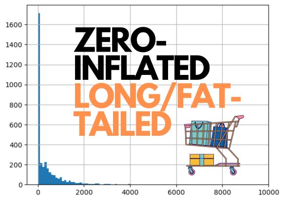
I have spent nearly a decade as a data scientist in the retail sector, but I have been approaching customer spend predictions the wrong way until I attended Gregory M. Duncan’s lecture. Accurately predicting how much an individual customer will spend in the next X days enables key retail use cases such as personalized promotion (determine X in Buy-X-Get-Y), customer targeting for upselling (which customers have higher purchasing power), and early churn detection (customers do not spend as much as they should). What makes this problem particularly difficult is because the distribution of customer spending is both zero-inflated and long/fat-tailed. Intuitively, most customers who visit your store are not going to make a purchase and among those who do, there will be some super customers who purchase an outrageous amount more than the average customer. Some parametric models allow for zero-inflated outcomes such as Poisson, negative binomial, Conway-Maxwell-Poisson; however, they do not handle the long/fat-tailed explicitly. Even for non-parametric models such as decision tree ensembles, more resources (trees and splits) will be dedicated to separating zeros and handling outliers; this could lead to deterioration in performance. Using the real-world dataset UCI Online Retail, we will compare the performance of common approaches namely naive baseline regression, regression on winsorized outcome, regression on log-plus-one-transformed outcome to what Duncan suggested: hurdle model with Duan’s method. We will demonstrate why this approach outperforms the others in most evaluation metrics and why it might not in some.

featured_image

import pandas as pd
import numpy as np
import random
from ucimlrepo import fetch_ucirepo 
import boto3
import json
from tqdm.auto import tqdm
import time
from sklearn.model_selection import train_test_split
from autogluon.tabular import TabularDataset, TabularPredictor
import seaborn as sns


from sklearn.metrics import (
    mean_squared_error, mean_absolute_error, r2_score, median_absolute_error,
    accuracy_score, precision_score, recall_score, f1_score, confusion_matrix
)
from scipy.stats import pearsonr, spearmanr, wasserstein_distance
from statsmodels.stats.diagnostic import het_white

def calculate_regression_metrics(y_true, y_pred):
    return {
        'root_mean_squared_error': np.sqrt(mean_squared_error(y_true, y_pred)),
        'mean_squared_error': mean_squared_error(y_true, y_pred),
        'mean_absolute_error': mean_absolute_error(y_true, y_pred),
        'r2': r2_score(y_true, y_pred),
        'pearsonr': pearsonr(y_true, y_pred)[0],
        'spearmanr': spearmanr(y_true, y_pred)[0],
        'median_absolute_error': median_absolute_error(y_true, y_pred),
        'earths_mover_distance': wasserstein_distance(y_true, y_pred)
    }

def caluclate_classification_metrics(y_true, y_pred):
    return {
        'accuracy': accuracy_score(y_true, y_pred),
        'precision': precision_score(y_true, y_pred, average='weighted'),
        'recall': recall_score(y_true, y_pred, average='weighted'),
        'f1_score': f1_score(y_true, y_pred, average='weighted'),
        'confusion_matrix': confusion_matrix(y_true, y_pred)
    }

def string_to_yearmon(date):
    date = date.split()
    date = date[0].split('/') + date[1].split(':')
    date = date[2] + '-' + date[0].zfill(2) #+ '-' + date[1].zfill(2) + ' ' + date[3].zfill(2) + ':' + date[4].zfill(2)
    return date

def call_llama(system_prompt, input):
    template = f"""<s>[INST] <<SYS>>{system_prompt}<</SYS>>{input}[/INST]"""
    client = boto3.client(service_name='bedrock-runtime',region_name='us-west-2')
    body = json.dumps({
        "prompt": template,
        "temperature": 0.,
        "top_p": 0.9,
        "max_gen_len": 2048,
    })
    response = client.invoke_model(
        body=body,
        modelId='us.meta.llama3-2-90b-instruct-v1:0',
        accept='application/json',
        contentType='application/json'
    )
    response_body = json.loads(response['body'].read())
    return response_body

def call_claude(system_prompt, input):
    client = boto3.client(service_name='bedrock-runtime',region_name='us-west-2')
    body=json.dumps(
        {
            "anthropic_version": "bedrock-2023-05-31",
            "max_tokens": 2048,
            "messages": [
                {
                    "role": "user",
                    "content": [
                    {
                        "type": "text",
                        "text": system_prompt + '\n' + input,
                    }
                    ]
                }
                ]
        }  
    )  

    
    response = client.invoke_model(body=body, 
                                   modelId='anthropic.claude-3-5-sonnet-20241022-v2:0',
                                   contentType='application/json',
                                   accept='application/json')
    response_body = json.loads(response.get('body').read())
   
    return response_body

This Is Not a Drill: Real-world Datasets, Meticulous Feature Engineering, State-of-the-art AutoML

To make this exercise as realistic as possible, we will use a real-world dataset (as opposed to a simulated one), perform as much feature engineering as we would in a real-world setting, and employ the best AutoML solution the market has to offer in AutoGluon.

online_retail = fetch_ucirepo(id=352) 
transaction_df = online_retail['data']['original']
original_nb = transaction_df.shape[0]

#create yearmon for train-valid split
transaction_df['yearmon'] = transaction_df.InvoiceDate.map(string_to_yearmon)

#get rid of transactions without cid
transaction_df = transaction_df[~transaction_df.CustomerID.isna()].reset_index(drop=True)
has_cid_nb = transaction_df.shape[0]

#fill in unknown descriptions
transaction_df.Description = transaction_df.Description.fillna('UNKNOWN')

#convert customer id to string
transaction_df['CustomerID'] = transaction_df['CustomerID'].map(lambda x: str(int(x)))

#simplify by filtering unit price and quantity to be non-zero (get rid of discounts, cancellations, etc)
transaction_df = transaction_df[(transaction_df.UnitPrice>0)&\
                                (transaction_df.Quantity>0)].reset_index(drop=True)
has_sales_nb = transaction_df.shape[0]

#add sales
transaction_df['Sales'] = transaction_df.UnitPrice * transaction_df.Quantity

We use the UCI Online Retail dataset, which contain transactions from a UK-based, non-store online retail from 2010-12 and 2011-12. We perform the following data processing:

1. Remove transactions without CustomerID; from 541,909 to 406,829 transactions
2. Filter out transactions where either UnitPrice or Quantity is less than zero; from 406,829 to 397,884 transactions
3. Fill in missing product Description with value UNKNOWN.

print(transaction_df.shape)
transaction_df.sample(5)

(397884, 10)

	InvoiceNo	StockCode	Description	Quantity	InvoiceDate	UnitPrice	CustomerID	Country	yearmon	Sales
276682	570008	22598	CHRISTMAS MUSICAL ZINC TREE	12	10/7/2011 9:30	0.85	13359	United Kingdom	2011-10	10.20
2894	536746	22604	SET OF 4 NAPKIN CHARMS CUTLERY	6	12/2/2010 13:39	2.55	16510	United Kingdom	2010-12	15.30
238815	566361	85123A	WHITE HANGING HEART T-LIGHT HOLDER	12	9/12/2011 12:32	2.95	15253	United Kingdom	2011-09	35.40
72407	545830	47590B	PINK HAPPY BIRTHDAY BUNTING	3	3/7/2011 13:10	5.45	17634	United Kingdom	2011-03	16.35
78138	546538	15044A	PINK PAPER PARASOL	6	3/14/2011 14:51	2.95	16327	United Kingdom	2011-03	17.70

We formulate the problem as predicting the sales (TargetSales) during Q4 2011 for each customers who bought at least one item during Q1-Q3 2011. Note that we are interested in predicting the spend per customer as accurately as possible; this is common for marketing use cases such as determining what spend threshold to give each customer in a promotion, targeting customers for upselling, or detecting early signs of churns. It is notably different from predicting total spend of all customers during a time period, which usually requires a different approach.

feature_period = {'start': '2011-01', 'end': '2011-09'}
outcome_period = {'start': '2011-10', 'end': '2011-12'}

feature_transaction = transaction_df[(transaction_df.yearmon>=feature_period['start'])&\
                                      (transaction_df.yearmon<=feature_period['end'])]
outcome_transaction = transaction_df[(transaction_df.yearmon>=outcome_period['start'])&\
                                      (transaction_df.yearmon<=outcome_period['end'])]

#aggregate sales during outcome period
outcome_sales = outcome_transaction.groupby('CustomerID').Sales.sum().reset_index()

#aggregate sales during feature period
feature_sales = feature_transaction.groupby('CustomerID').Sales.sum().reset_index()

#merge to get TargetSales including those who spent during feature period but not during outcome (zeroes)
outcome_df = feature_sales[['CustomerID']].merge(outcome_sales, on='CustomerID', how='left')
outcome_df['Sales'] = outcome_df['Sales'].fillna(0)
outcome_df.columns = ['CustomerID', 'TargetSales']

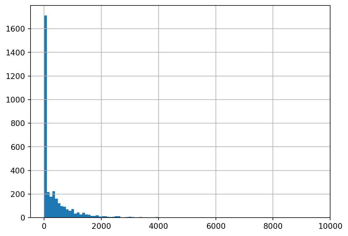
We transform the transaction dataset into a customer-level dataset where we calculate features using transactions between 2011-01 to 2011-09 and outcome using transactions between 2011-10 to 2011-12, summing Quantity times UnitPrice. We left-join the customers in feature set to outcome set. This will result in the zero-inflated nature of the outcome as not all customers will come back in Q4. The distribution of non-zero sales is naturally long/fat-tailed with a few customers having extraordinarily high amount of sales in Q4. This resulted in a customer-level dataset with 3,438 customers.

#confirm zero-inflated, long/fat-tailed
outcome_df.TargetSales.describe(percentiles=[i/10 for i in range(10)])

count      3438.000000
mean        666.245829
std        4016.843037
min           0.000000
0%            0.000000
10%           0.000000
20%           0.000000
30%           0.000000
40%           0.000000
50%         102.005000
60%         263.006000
70%         425.790000
80%         705.878000
90%        1273.611000
max      168469.600000
Name: TargetSales, dtype: float64

#confirm zero-inflated, long/fat-tailed
outcome_df[outcome_df.TargetSales<=10_000].TargetSales.hist(bins=100)

We represent a customer using traditional RFM features namely recency of purchase, purchase days, total sales, number of distinct products purchased, number of distinct category purchased, customer tenure within 2011, average purchase frequency, average purchase value, and percentage of purchase across all 9 categories. This is based on data from Q1-Q3 2011.

Since the UCI Online Retail dataset does not have a category but only contains descriptions over 3,000 items, we use LLaMA 3.2 90B to infer categories based on randomly selected 1,000 descriptions. This is to make the category preference representation for each customer, which is more tractable than including features about all 3,548 items. After that, we use Claude 3.5 v2 to label a category for each description as it performs structured output a little more reliably. The categories are:

1. Home Decor
2. Kitchen and Dining
3. Fashion Accessories
4. Stationary and Gifts
5. Toys and Games
6. Seasonal and Holiday
7. Personal Care and Wellness
8. Outdoor and Garden
9. Others

descriptions = feature_transaction.Description.unique().tolist()
print(descriptions[:5])

#randomize descriptions with seed 112 to get which categories we should use
np.random.seed(112)
random_descriptions = np.random.choice(descriptions, 1000, replace=False)

res = call_llama(
    'You are a product categorization assistant at a retail website.',
    'Given the following product descriptions, come up with a few product categories they should be classified into.'+'\n'.join(random_descriptions)
)

categories = [
    'Home Decor',
    'Kitchen and Dining',
    'Fashion Accessories',
    'Stationary and Gifts',
    'Toys and Games',
    'Seasonal and Holiday',
    'Personal Care and Wellness',
    'Outdoor and Garden',   
]

print(res['generation'])

['JUMBO BAG PINK POLKADOT', 'BLUE POLKADOT WRAP', 'RED RETROSPOT WRAP ', 'RECYCLING BAG RETROSPOT ', 'RED RETROSPOT SHOPPER BAG']
 <<SYS>>Based on the product descriptions, I would categorize them into the following categories:

1. Home Decor:
    * Wall art
    * Decorative items (e.g. vases, figurines, etc.)
    * Lighting (e.g. candles, lanterns, etc.)
    * Textiles (e.g. throw pillows, blankets, etc.)
2. Kitchen and Dining:
    * Cookware and utensils
    * Tableware (e.g. plates, cups, etc.)
    * Kitchen decor (e.g. signs, magnets, etc.)
    * Food and drink items (e.g. tea, coffee, etc.)
3. Fashion and Accessories:
    * Jewelry (e.g. necklaces, earrings, etc.)
    * Handbags and wallets
    * Clothing and accessories (e.g. scarves, hats, etc.)
    * Beauty and personal care items (e.g. cosmetics, skincare, etc.)
4. Stationery and Gifts:
    * Greeting cards
    * Gift wrap and bags
    * Stationery (e.g. notebooks, pens, etc.)
    * Gift items (e.g. mugs, keychains, etc.)
5. Toys and Games:
    * Toys (e.g. stuffed animals, puzzles, etc.)
    * Games and puzzles
    * Outdoor toys and games
6. Seasonal and Holiday:
    * Christmas decorations and gifts
    * Easter decorations and gifts
    * Halloween decorations and gifts
    * Other seasonal and holiday items
7. Office and School:
    * Office supplies (e.g. pens, paper, etc.)
    * School supplies (e.g. backpacks, lunchboxes, etc.)
    * Desk accessories (e.g. paperweights, etc.)
8. Garden and Outdoor:
    * Gardening tools and supplies
    * Outdoor decor (e.g. planters, etc.)
    * Patio and outdoor furniture
9. Baby and Kids:
    * Baby clothing and accessories
    * Kids' clothing and accessories
    * Toys and games for kids
    * Nursery decor and furniture

Note that some products may fit into multiple categories, but I've tried to categorize them based on their primary function or theme.

#loop through descriptions in batches of batch_size
res_texts = []
batch_size = 100
for i in tqdm(range(0, len(descriptions), batch_size)):
    batch = descriptions[i:i+batch_size]
    d = "\n".join(batch)
    inp = f'''Categorize the following product descriptions into {", ".join(categories)} or Others, if they do not fall into any. 
Only answer in the following format:

"product description of product #1"|"product category classified into"
"product description of product #2"|"product category classified into"
...
"product description of product #n"|"product category classified into"

Here are the product descriptions:
{d}
'''
    while True:
        res = call_claude('You are a product categorizer at a retail website', inp)
        # if res['generation_token_count'] > 1: #for llama
        if res['usage']['output_tokens'] > 1:
            break
        else:
            print('Retrying...')
            time.sleep(2)
    res_text = res['content'][0]['text'].strip().split('\n')
        #for llama
        # .replace('[SYS]','').replace('<<SYS>>','')\
        # .replace('[/SYS]','').replace('<</SYS>>','')\
    if res_text!='':
        res_texts.extend(res_text)

with open('../../data/sales_prediction/product_description_category.csv','w') as f:
    f.write('"product_description"|"category"\n')
    for i in res_texts:
        f.write(f'{i}\n')

Here is the share of product descriptions in each annotated category:

product_description_category = pd.read_csv('../../data/sales_prediction/product_description_category.csv',
                                           sep='|')

#clean product_description
product_description_category['Description'] = descriptions
product_description_category.category.value_counts(normalize=True)

category
Home Decor                    0.328636
Kitchen and Dining            0.195885
Fashion Accessories           0.138670
Stationary and Gifts          0.116122
Seasonal and Holiday          0.087373
Personal Care and Wellness    0.047351
Toys and Games                0.045096
Outdoor and Garden            0.032976
Others                        0.007892
Name: proportion, dtype: float64

We merge the RFM features with preference features, that is share of sales in each category for every customer, then the outcome TargetSales to create the universe set for the problem.

feature_transaction_cat = feature_transaction.merge(product_description_category,
                                                    how='inner',
                                                    on = 'Description',)
feature_transaction.shape, feature_transaction_cat.shape

#convert invoice date to datetime
feature_transaction_cat['InvoiceDate'] = pd.to_datetime(feature_transaction_cat['InvoiceDate'])

# last date in feature set
current_date = feature_transaction_cat['InvoiceDate'].max()

#rfm
customer_features = feature_transaction_cat.groupby('CustomerID').agg({
    'InvoiceDate': [
        ('recency', lambda x: (current_date - x.max()).days),
        ('first_purchase_date', 'min'),
        ('purchase_day', 'nunique'),
    ],
    'InvoiceNo': [('nb_invoice', 'nunique')],
    'Sales': [
        ('total_sales', 'sum')
    ],
    'StockCode': [('nb_product', 'nunique')],
    'category': [('nb_category', 'nunique')]
}).reset_index()

# Flatten column names
customer_features.columns = [
    'CustomerID',
    'recency',
    'first_purchase_date',
    'purchase_day',
    'nb_invoice',
    'total_sales',
    'nb_product',
    'nb_category'
]

customer_features['customer_lifetime'] = (current_date - customer_features['first_purchase_date']).dt.days
customer_features['avg_purchase_frequency'] = customer_features['customer_lifetime'] / customer_features['purchase_day']
customer_features['avg_purchase_value'] = customer_features['total_sales'] / customer_features['purchase_day']

#category preference
category_sales = feature_transaction_cat.pivot_table(
    values='Sales', 
    index='CustomerID', 
    columns='category', 
    aggfunc='sum', 
    fill_value=0
)
category_sales.columns = [i.lower().replace(' ','_') for i in category_sales.columns]
customer_features = customer_features.merge(category_sales, on='CustomerID', how='left')

total_sales = customer_features['total_sales']
for col in category_sales.columns:
    percentage_col = f'per_{col}'
    customer_features[percentage_col] = customer_features[col] / total_sales

selected_features = [
 'recency',
 'purchase_day',
 'total_sales',
 'nb_product',
 'nb_category',
 'customer_lifetime',
 'avg_purchase_frequency',
 'avg_purchase_value',
 'per_fashion_accessories',
 'per_home_decor',
 'per_kitchen_and_dining',
 'per_others',
 'per_outdoor_and_garden',
 'per_personal_care_and_wellness',
 'per_seasonal_and_holiday',
 'per_stationary_and_gifts',
 'per_toys_and_games']

outcome_variable = 'TargetSales'

customer_features = customer_features[[ 'CustomerID']+selected_features]
df = outcome_df.merge(customer_features, on='CustomerID').drop('CustomerID', axis=1)
print(df.shape)
df.sample(5)

(3438, 18)

	TargetSales	recency	purchase_day	total_sales	nb_product	nb_category	customer_lifetime	avg_purchase_frequency	avg_purchase_value	per_fashion_accessories	per_home_decor	per_kitchen_and_dining	per_others	per_outdoor_and_garden	per_personal_care_and_wellness	per_seasonal_and_holiday	per_stationary_and_gifts	per_toys_and_games
2606	0.00	53	2	597.48	138	8	184	92.000000	298.740	0.079383	0.433973	0.343710	0.003465	0.000000	0.041357	0.016570	0.056688	0.024854
196	0.00	78	2	2209.85	37	6	226	113.000000	1104.925	0.030771	0.275245	0.628549	0.000000	0.021178	0.022535	0.000000	0.021721	0.000000
2900	3893.79	10	6	4099.11	78	9	172	28.666667	683.185	0.003879	0.761507	0.104540	0.003879	0.012442	0.014015	0.051597	0.043312	0.004830
2187	0.00	227	1	122.40	1	1	227	227.000000	122.400	0.000000	0.000000	1.000000	0.000000	0.000000	0.000000	0.000000	0.000000	0.000000
322	0.00	68	1	147.12	3	2	68	68.000000	147.120	0.881729	0.118271	0.000000	0.000000	0.000000	0.000000	0.000000	0.000000	0.000000

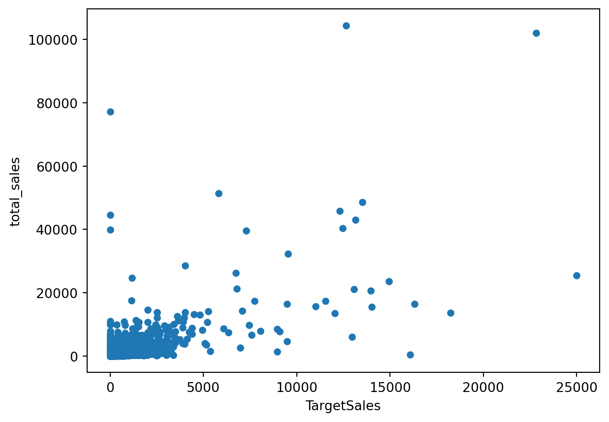
Univariate correlation expectedly pinpoints total_sales in during Q1-Q3 2011 as the most predictive feature; however, we can see that it is still not very predictive. This shows that the problem is not a trivial one.

print(df[['TargetSales','total_sales']].corr())

#target and most predictive variable
df[df.TargetSales<=25_000].plot.scatter(x='TargetSales',y='total_sales')

             TargetSales  total_sales
TargetSales     1.000000     0.558558
total_sales     0.558558     1.000000

We randomly split the dataset into train and test sets at 80/20 ratio. We also confirm the distribution of TargetSales is similar across percentiles between train and test and only different at the upper end.

#split into train-valid sets
train_df, test_df = train_test_split(df,
                                      test_size=0.2, 
                                      random_state=112)
pd.concat([train_df.TargetSales.describe(percentiles=[i/10 for i in range(10)]).reset_index(),
test_df.TargetSales.describe(percentiles=[i/10 for i in range(10)]).reset_index(),], axis=1)

	index	TargetSales	index	TargetSales
0	count	2750.000000	count	688.000000
1	mean	642.650436	mean	760.558808
2	std	4015.305436	std	4024.524400
3	min	0.000000	min	0.000000
4	0%	0.000000	0%	0.000000
5	10%	0.000000	10%	0.000000
6	20%	0.000000	20%	0.000000
7	30%	0.000000	30%	0.000000
8	40%	0.000000	40%	0.000000
9	50%	91.350000	50%	113.575000
10	60%	260.308000	60%	277.836000
11	70%	426.878000	70%	418.187000
12	80%	694.164000	80%	759.582000
13	90%	1272.997000	90%	1255.670000
14	max	168469.600000	max	77099.380000

Naive Baseline Regression

The most naive solution is to simply predict TargetSales based on the features. We use a stacked ensemble of LightGBM, CatBoost, XGBoost, Random Forest and Extra Trees via AutoGluon. We train with good_quality preset, stated to be “Stronger than any other AutoML Framework”, for speedy training and inference but feel free to try more performant options. We exclude the neural-network models as they require further preprocessing of the features. We use an industry-grade, non-parametric model to be as close to a real use case as possible and make a point that the methodology works not only in a toy-dataset setup.

preset = 'good_quality'

predictor = TabularPredictor(label='TargetSales').fit(train_df[selected_features + ['TargetSales']], 
                                                      presets=preset,
                                                      excluded_model_types=['NN_TORCH','FASTAI','KNN'],
                                                      )
test_df['pred_baseline'] = predictor.predict(test_df[selected_features])

metric_baseline = calculate_regression_metrics(test_df['TargetSales'], test_df['pred_baseline'])
metric_baseline['model'] = 'baseline'
metric_baseline

{'root_mean_squared_error': 3162.478744240967,
 'mean_squared_error': 10001271.807775924,
 'mean_absolute_error': 715.6442657130541,
 'r2': 0.3816166296854987,
 'pearsonr': 0.6190719671013133,
 'spearmanr': 0.47008461549340863,
 'median_absolute_error': 232.98208312988282,
 'earths_mover_distance': 287.77728784026124,
 'model': 'baseline'}

Regression on Winsorized Outcome

outlier_per = 0.99
outlier_cap_train = train_df['TargetSales'].quantile(outlier_per)

An alternative approach to deal with long/fat-tailed outcome is to train on a winsorized outcome. In our case, we cap the outlier at 99.0% or TargetSales equals 7,180.81. While this solves the long/fat-tailed issues, it does not deal with zero inflation and also introduce bias to the outcome. This leads to better performance when tested on the winsorized outcome, but not so much on the original outcome.

#winsorize
train_df['TargetSales_win'] = train_df['TargetSales'].map(lambda x: outlier_cap_train if x> outlier_cap_train else x)
test_df['TargetSales_win'] = test_df['TargetSales'].map(lambda x: outlier_cap_train if x> outlier_cap_train else x)

predictor = TabularPredictor(label='TargetSales_win').fit(train_df[selected_features+['TargetSales_win']],
                                                      presets=preset,
                                                      excluded_model_types=['NN_TORCH','FASTAI','KNN'],
                                                      )

test_df['pred_winsorized'] = predictor.predict(test_df[selected_features])

metric_winsorized = calculate_regression_metrics(test_df['TargetSales'], test_df['pred_winsorized'])
metric_winsorized['model'] = 'winsorized'
metric_winsorized

{'root_mean_squared_error': 3623.576377551195,
 'mean_squared_error': 13130305.76394704,
 'mean_absolute_error': 627.7880071099414,
 'r2': 0.18814697894155963,
 'pearsonr': 0.5757989413256978,
 'spearmanr': 0.504301956183441,
 'median_absolute_error': 219.62248107910156,
 'earths_mover_distance': 432.1288432991232,
 'model': 'winsorized'}

Regression on Log-plus-one-transformed Outcome

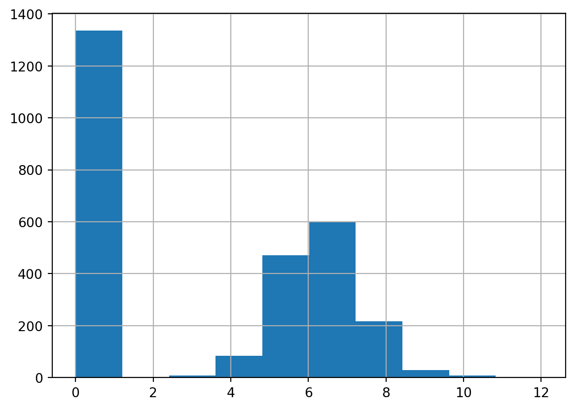
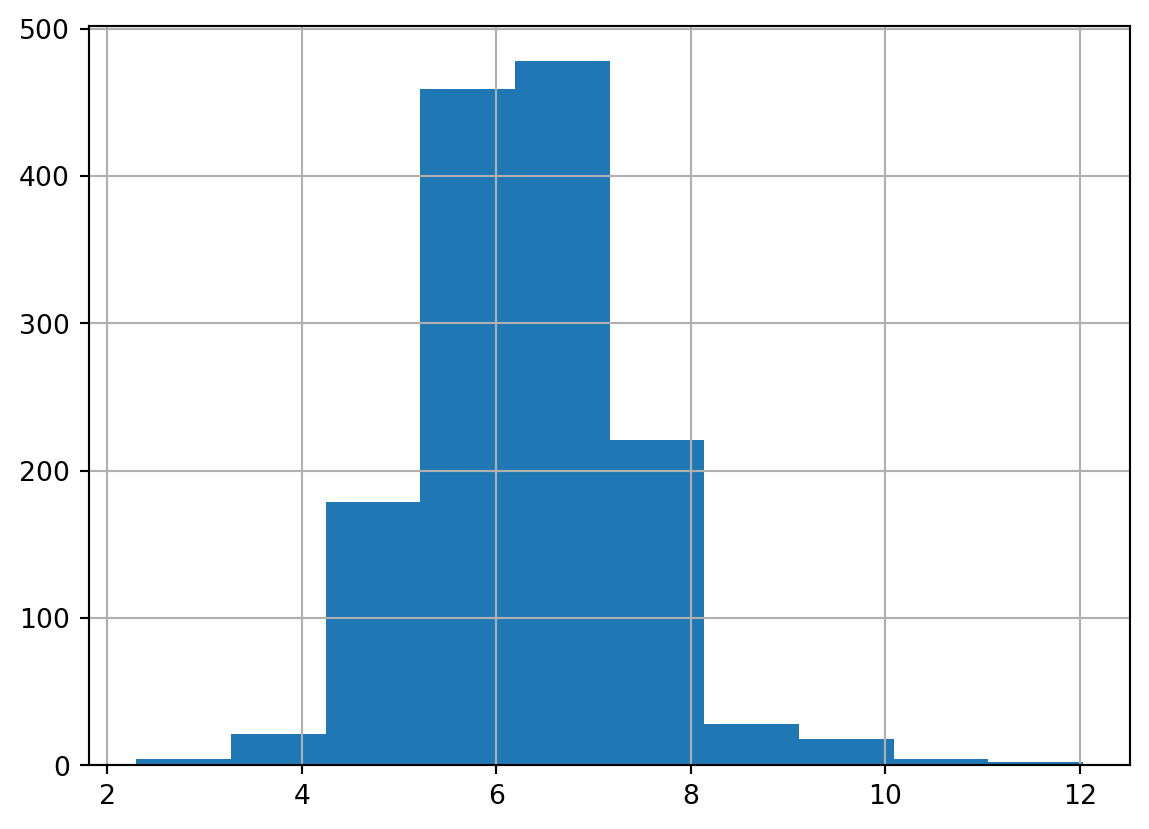
Log transformation handles long/fat-tailed distribution and is especially useful for certain models since the transformed distribution is closer normal. However, it cannot handle zero-valued outcome and oftentimes scientists end up adding 1 to the outcome (so often that numpy even has a function for it). This not only introduces bias to the prediction, but also does not solve the zero-inflation as it becomes one-inflation instead.

#log
train_df['TargetSales_log1p'] = train_df['TargetSales'].map(np.log1p)
test_df['TargetSales_log1p'] = test_df['TargetSales'].map(np.log1p)

#from zero-inflated to one-inflated
train_df['TargetSales_log1p'].hist()

We can see that this is the best performing approach so far, which is one of the reasons why so many scientists end up going for this not-entirely-correct approach.

predictor = TabularPredictor(label='TargetSales_log1p').fit(train_df[selected_features+['TargetSales_log1p']],
                                                      presets=preset,
                                                      excluded_model_types=['NN_TORCH','FASTAI','KNN'],
                                                      )

test_df['pred_log1p'] = predictor.predict(test_df[selected_features])
test_df['pred_log1p_expm1'] = test_df['pred_log1p'].map(np.expm1)

metric_log1p = calculate_regression_metrics(test_df['TargetSales'], test_df['pred_log1p_expm1'])
metric_log1p['model'] = 'log1p'
metric_log1p

{'root_mean_squared_error': 3725.342295894091,
 'mean_squared_error': 13878175.221577456,
 'mean_absolute_error': 618.9768466651894,
 'r2': 0.14190585634701047,
 'pearsonr': 0.5817166874396966,
 'spearmanr': 0.5338156315937898,
 'median_absolute_error': 89.55495441784018,
 'earths_mover_distance': 581.0494444960044,
 'model': 'log1p'}

Hurdle Model

Hurdle model is a two-stage approach that handles zero inflation by first having a classification model to predict if the outcome is zero or not, then a regression model, trained only on examples with actual non-zero outcomes, to fit a log-transformed outcome. When retransforming the predictions from log to non-log numbers, we perform correction of underestimation using Duan’s method. During inference time, we multiply the predictions from the classification and corrected regression model.

train_df['has_purchase'] = train_df.TargetSales.map(lambda x: 1 if x>0 else 0)
test_df['has_purchase'] = test_df.TargetSales.map(lambda x: 1 if x>0 else 0)

predictor_cls = TabularPredictor(label='has_purchase').fit(train_df[selected_features+['has_purchase']],
                                                      presets=preset,
                                                      excluded_model_types=['NN_TORCH','FASTAI','KNN'],
                                                      )
test_df['pred_binary'] = predictor_cls.predict(test_df[selected_features])

For our splits, 51.42% of train and 53.05% of test include customers with non-zero purchase outcome. As with all two-stage approaches, we need to make sure the intermediate model performs reasonably in classifying zero/non-zero outcomes.

caluclate_classification_metrics(test_df['has_purchase'], test_df['pred_binary'])

{'accuracy': 0.6918604651162791,
 'precision': 0.6941069004479309,
 'recall': 0.6918604651162791,
 'f1_score': 0.6921418829824787,
 'confusion_matrix': array([[229,  94],
        [118, 247]])}

train_df_nonzero = train_df[train_df.has_purchase==1].reset_index(drop=True)
test_df_nonzero = test_df[test_df.has_purchase==1].reset_index(drop=True)

#log
train_df_nonzero['TargetSales_log'] = train_df_nonzero['TargetSales'].map(np.log)
test_df_nonzero['TargetSales_log'] = test_df_nonzero['TargetSales'].map(np.log)

After that, we perform log-transformed regression on the examples with non-zero outcome (1,414 examples in train). Without the need to worry about ln(0) outcome, the regression is much more straightforward albeit with fewer examples to train on.

train_df_nonzero['TargetSales_log'].hist()

predictor_reg = TabularPredictor(label='TargetSales_log').fit(train_df_nonzero[selected_features+['TargetSales_log']],
                                                      presets=preset,
                                                      excluded_model_types=['NN_TORCH','FASTAI','KNN'],
                                                      )
test_df_nonzero['pred_log'] = predictor_reg.predict(test_df_nonzero[selected_features])
test_df_nonzero['pred_log_exp'] = test_df_nonzero['pred_log'].map(np.exp)

test_df['pred_log'] = predictor_reg.predict(test_df[selected_features])
test_df['pred_log_exp'] = test_df['pred_log'].map(np.exp)

test_df['pred_hurdle'] = test_df.pred_binary * test_df.pred_log_exp

For inference, we combine the binary prediction (purchase/no purchase) from the classification model with the re-transformed (exponentialized) numerical prediction from the regression model by simply multiplying them together. As you can see, this approach yields the best performance so far and this is where I used to think everything has been accounted for.

metric_hurdle = calculate_regression_metrics(test_df['TargetSales'], test_df['pred_hurdle'])
metric_hurdle['model'] = 'hurdle'
metric_hurdle

{'root_mean_squared_error': 3171.760744960863,
 'mean_squared_error': 10060066.22327469,
 'mean_absolute_error': 584.9162934881963,
 'r2': 0.3779813431428882,
 'pearsonr': 0.6769697889999318,
 'spearmanr': 0.5107083593715698,
 'median_absolute_error': 199.1780137692856,
 'earths_mover_distance': 286.381442541919,
 'model': 'hurdle'}

But Wait, There Is MoreーEnter Naihua Duan

In the previous section, we have blissfully assumed that we can freely log-transform and re-transform the outcome during training and inference without any bias. This is not the case as there is a small bias generated in the process due to the error term.

\[ln(y) = f(X) + \epsilon\]

where

• \(y\) is actual outcome.

• \(X\) is the features.

• \(f(.)\) is a trained model.

• \(\epsilon\) is the error term.

when re-transforming

\[ \begin{align} y &= exp(ln(y)) \\ &= exp(f(X) + \epsilon ) \\ &= exp(f(X)) \cdot exp(\epsilon) \\ E[y] &= E[exp(f(X))] \cdot E[exp(\epsilon)] \end{align} \]

The average treatment affect (ATE; \(E[y]\)) is underestimated by \(E[exp(\epsilon)]\). Naihua Duan (段乃華), a Taiwanese biostatistician, suggested a consistent estimator of \(E[exp(\epsilon)]\) in his 1983 work as

\[ \begin{align} \hat \lambda &= E[exp(ln(y) - ln(\hat y))] \end{align} \]

where

• \(\hat \lambda\) is the Duan’s smearing estimator of the bias from re-transformation \(E[exp(\epsilon)]\)

• \(\hat y\) is the prediction aka \(f(X)\)

Fun Fact: If you assume Duan were a western name, you would have been 
pronouncing the method's name incorrectly since it should be [twàn]'s 
method, NOT /dwɑn/'s method.

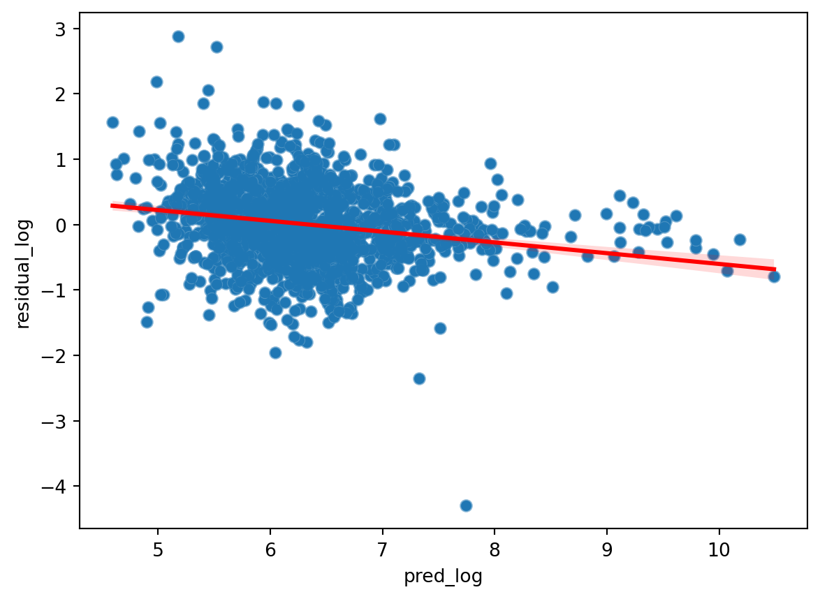
Before we proceed, the formulation of Duan’s smearing estimator assumes that estimates of error terms (residuals) for log predictions be independent and identically distributed. Since we are dealing with individual customers, independence can be assumed. However, if we look at the plot of residuals vs predicted log values (based on training set), we can see that they do not look particularly identically distributed.

#plot residual and predicted log value
train_df_nonzero['pred_log'] = predictor_reg.predict(train_df_nonzero[selected_features])
train_df_nonzero['residual_log'] = (train_df_nonzero['pred_log'] - train_df_nonzero['TargetSales_log'])

# Create the scatter plot
sns.scatterplot(x='pred_log', y='residual_log', data=train_df_nonzero)

# Add the Lowess smoothing line
sns.regplot(x='pred_log', y='residual_log', data=train_df_nonzero, scatter_kws={'alpha': 0.5}, line_kws={'color': 'red'})

Although note that White test does not reject the null hypothesis of the residuals being homoscedastic in reference to the features. This counterintuitive result might stem from the fact that White test is assuming linear or quadratic relationships between outcome and features while the residuals are derived from a stacked ensemble of decision trees.

white_stat, white_p_value, _, _ = het_white(train_df_nonzero['residual_log'], 
                                            train_df_nonzero[selected_features])
print(f"White Test Statistic: {white_stat}")
print(f"P-value: {white_p_value}")

White Test Statistic: 129.31318320644837
P-value: 0.8761278601130765

Our choice is to either trust the White test and pretend assume everything is fine; or trust our eyes and replace the non-zero regression model with one that produces iid residuals such as generalized least squares (GLS) with heteroscedasticity-robust standard errors. The tradeoff is that often models that produce homoscedastic residuals perform worse in terms of predictive power (see example of GLS implementation in Assumption on Indepedent and Identically Distributed Residuals section of the notebook).

Assuming we trust the White test, we can easily derive Duan’s smearing estimator by taking mean of error between actual and predicted TargetSales in the training set.

train_df_nonzero['pred_log'] = predictor_reg.predict(train_df_nonzero[selected_features])
train_df_nonzero['pred_log_exp'] = train_df_nonzero['pred_log'].map(np.exp)

smearing_estimator = np.mean(np.exp(train_df_nonzero['TargetSales_log'] - train_df_nonzero['pred_log']))
smearing_estimator

1.2280991653046711

We multiply this to the predictions of the hurdle model to correct the underestimation due to re-transformation bias.

test_df['pred_log_exp_corrected'] = test_df['pred_log_exp'] * smearing_estimator
test_df['pred_hurdle_corrected'] = test_df.pred_binary * test_df.pred_log_exp_corrected

metric_hurdle_corrected = calculate_regression_metrics(test_df['TargetSales'], test_df['pred_hurdle_corrected'])
metric_hurdle_corrected['model'] = 'hurdle_corrected'
metric_hurdle_corrected

{'root_mean_squared_error': 3055.3207868281233,
 'mean_squared_error': 9334985.110424023,
 'mean_absolute_error': 613.3946643257099,
 'r2': 0.42281345159207295,
 'pearsonr': 0.6769697889999318,
 'spearmanr': 0.5107083593715698,
 'median_absolute_error': 232.55557358084502,
 'earths_mover_distance': 241.61839859133218,
 'model': 'hurdle_corrected'}

The Eval Bar

We can see that the hurdle model with Duan’s correction performs best across majority of the metrics. We will now deep dive on metrics where it did not to understand the caveats when taking this approach.

metric_df = pd.DataFrame([metric_baseline,
                       metric_winsorized,
                       metric_log1p,
                       metric_hurdle,
                       metric_hurdle_corrected,])

rank_df = metric_df.copy()
for col in metric_df.columns.tolist()[:-1]:
    if col in ['r2', 'pearsonr', 'spearmanr']:
        rank_df[f'{col}_rank'] = rank_df[col].rank(ascending=False)
    else:
        rank_df[f'{col}_rank'] = rank_df[col].rank(ascending=True)
rank_df = rank_df.drop(metric_df.columns.tolist()[:-1], axis=1)
rank_df['avg_rank'] = rank_df.iloc[:,1:].mean(axis=1)
rank_df.transpose()

	0	1	2	3	4
model	baseline	winsorized	log1p	hurdle	hurdle_corrected
root_mean_squared_error_rank	2.0	4.0	5.0	3.0	1.0
mean_squared_error_rank	2.0	4.0	5.0	3.0	1.0
mean_absolute_error_rank	5.0	4.0	3.0	1.0	2.0
r2_rank	2.0	4.0	5.0	3.0	1.0
pearsonr_rank	3.0	5.0	4.0	1.5	1.5
spearmanr_rank	5.0	4.0	1.0	2.5	2.5
median_absolute_error_rank	5.0	3.0	1.0	2.0	4.0
earths_mover_distance_rank	3.0	4.0	5.0	2.0	1.0
avg_rank	3.375	4.0	3.625	2.25	1.75

metric_df.transpose()

	0	1	2	3	4
root_mean_squared_error	3162.478744	3623.576378	3725.342296	3171.760745	3055.320787
mean_squared_error	10001271.807776	13130305.763947	13878175.221577	10060066.223275	9334985.110424
mean_absolute_error	715.644266	627.788007	618.976847	584.916293	613.394664
r2	0.381617	0.188147	0.141906	0.377981	0.422813
pearsonr	0.619072	0.575799	0.581717	0.67697	0.67697
spearmanr	0.470085	0.504302	0.533816	0.510708	0.510708
median_absolute_error	232.982083	219.622481	89.554954	199.178014	232.555574
earths_mover_distance	287.777288	432.128843	581.049444	286.381443	241.618399
model	baseline	winsorized	log1p	hurdle	hurdle_corrected

Why Duan’s Correction Results in Slightly Worse MAE?

Duan’s method adjusts for underestimation from re-transformation of log outcome. This could lead to smaller extreme errors, but more frequent occurrences of less extreme ones. We verify this hypothesis by comparing mean absolute error before and after transformation for errors originally under and over 99th percentile. We confirm that is the case for our problem.

err_hurdle = (test_df['TargetSales'] - test_df['pred_hurdle']).abs()
err_hurdle_corrected = (test_df['TargetSales'] - test_df['pred_hurdle_corrected']).abs()

print('Distribution of errors for Hurdle model without correction')
err_hurdle.describe(percentiles=[.25, .5, .75, .9, .95, .99]) 

Distribution of errors for Hurdle model without correction

count      688.000000
mean       584.916293
std       3119.628924
min          0.000000
25%          0.000000
50%        199.178014
75%        475.603446
90%        862.530026
95%       1237.540954
99%       6763.777844
max      55731.205996
dtype: float64

print('Hurdle Model without correction')
print(f'Mean absolute error under 99th percentile: {err_hurdle[err_hurdle<6763.777844].mean()}')
print(f'Mean absolute error over 99th percentile: {err_hurdle[err_hurdle>6763.777844].mean()}')

print('Hurdle Model with correction')
print(f'Mean absolute error under 99th percentile: {err_hurdle_corrected[err_hurdle<6763.777844].mean()}')
print(f'Mean absolute error over 99th percentile: {err_hurdle_corrected[err_hurdle>6763.777844].mean()}')

Hurdle Model without correction
Mean absolute error under 99th percentile: 355.4918014848842
Mean absolute error over 99th percentile: 22904.641872667555
Hurdle Model with correction
Mean absolute error under 99th percentile: 392.7718802742851
Mean absolute error over 99th percentile: 22076.839798471465

Importance of Classification Model

The overperformance of log-transform regression over both hurdle model approarches in Spearman’s rank correlation and median absolute error demonstrates the importance of a classification model. At first glance, it is perplexing since we have just spent a large portion of this article to justify that hurdle models handle zero inflation better and re-transformation without Duan’s method is biased. However, it becomes clear once you compare performance of the hurdle model with a classification model (f1 = 0.69) and a hypothetical, perfect classification model. Other metrics also improved but not nearly as drastic as MedAE and Spearman’s rank correlation.

test_df['pred_hurdle_corrected_perfect_cls'] = test_df.has_purchase * test_df.pred_log_exp_corrected
metric_hurdle_corrected_perfect_cls = calculate_regression_metrics(test_df['TargetSales'], test_df['pred_hurdle_corrected_perfect_cls'])
metric_hurdle_corrected_perfect_cls['model'] = 'hurdle_corrected_perfect_cls'

metric_df2 = pd.DataFrame([metric_baseline,
                       metric_winsorized,
                       metric_log1p,
                       metric_hurdle,
                       metric_hurdle_corrected,
                       metric_hurdle_corrected_perfect_cls,])
metric_df2.transpose()

	0	1	2	3	4	5
root_mean_squared_error	3162.478744	3623.576378	3725.342296	3171.760745	3055.320787	3030.854831
mean_squared_error	10001271.807776	13130305.763947	13878175.221577	10060066.223275	9334985.110424	9186081.006625
mean_absolute_error	715.644266	627.788007	618.976847	584.916293	613.394664	479.558294
r2	0.381617	0.188147	0.141906	0.377981	0.422813	0.43202
pearsonr	0.619072	0.575799	0.581717	0.67697	0.67697	0.687639
spearmanr	0.470085	0.504302	0.533816	0.510708	0.510708	0.929419
median_absolute_error	232.982083	219.622481	89.554954	199.178014	232.555574	34.991964
earths_mover_distance	287.777288	432.128843	581.049444	286.381443	241.618399	234.587018
model	baseline	winsorized	log1p	hurdle	hurdle_corrected	hurdle_corrected_perfect_cls

Remember What Problem We Are Solving

One last thing to remember is that we are trying to predict sales of each individual customer, not total sales of all customers. If we look at aggregated mean or sum of actual sales vs predicted sales, baseline regression performs best by far. This is due to the fact that without any constraints a regressor only minimizes the MSE loss and usually ends up predicting values around the mean to balance between under- and over-predictions. However, this level of prediction is often not very useful as a single point. Imagine you want to give promotions with higher or lower spend thresholds to customers according to their purchasing power; you will not be able to do so with a model that is accurate on aggregate but not so much on individual customers.

test_df[['TargetSales','pred_baseline','pred_winsorized','pred_log1p_expm1','pred_hurdle','pred_hurdle_corrected']].mean()

TargetSales              760.558808
pred_baseline            791.043945
pred_winsorized          508.281555
pred_log1p_expm1         186.200281
pred_hurdle              527.286811
pred_hurdle_corrected    647.560493
dtype: float64

Closing Remarks

And this is how you predict how much a customer will spend in the least wrong way. My hope is that you will not need to spend ten years in data science to find out how to do it like I did.